 |
in electric arcs.
In P. Pisarczyk, T. Pisarczyk and J. Wolowski (Ed.):
Proceedings of the XXIV International Conference
on Phenomena in Ionized Gases,
Warschau, Polen, 11-16 July 1999
(ISBN 83-902319-5-6), Bd.II, S.227-228
(best computational poster award)
Modeling of arc-electrode systems
- preliminary results for high pressure xenon arc lamps.
8th Int. Symposium on the Science & Technology of
Light Sources (LS-8), Greifswald,
30.8.-3.9.1998 (ISBN 3-00-003105-7), S.382-383
In: G. Babucke (ed.),
XII Int. Conf. Gas Discharges and their Applications,
Greifswald,
8.-12.9.1997 (ISBN 3-00-001760-7), Bd.I (1997), S.62-65
In: H. Cerjak (ed.),
Mathematical Modelling of Weld Phenomena 3
(ISBN 1-86125-010-X),
The Institute of Materials, London, 1997, S.848-897
Berechnung anwendungsrelevanter Zielgrößen
von thermischen Lichtbögen:
Kathodenfallmodelle und deren Integration
in die Lichtbogenmodellierung.
8te Bundesdeutsche Fachtagung Plasmatechnologie,
Dresden, 14-17.7.1997, S.17
Modellierung thermischer Lichtbögen zur
Optimierung von technologischen Prozeßparametern.
7te Bundesdeutsche Fachtagung Plasmatechnologie,
Bochum 13-14.3.1996, S.118
Modellierung des Kathodenfalls zur Simulation thermischer
Lichtbögen.
7te Bundesdeutsche Fachtagung Plasmatechnologie,
Bochum 13-14.3.1996, S.37
Modellierung der katodennahen Plasmarandschichten eines
WIG-Lichtbogens.
Verhandl. DPG (VI) Bd.30 (1995), S.243
dedicated
*23.1.1930 f11.2.2000
to
Prof. Dr. Gerhard Simon
Thermische Plasmen wurden in Form von Lichtbogenentladungen Anfang des neunzehnten Jahrhunderts entdeckt. Die fundamentalen physikalischen Mechanismen dieser Gasentladungen wurden bereits im Jahre 1903 von J. Stark beschrieben. Während die grundlegende Physik dieses Phänomens somit weitgehend bekannt ist, war es bis heute praktisch kaum möglich, wesentliche Entladungsparameter quantitativ vorauszuberechnen.
Ein fundamentales Problem der Modellierung lag in der Beschreibung der Nichtgleichgewichtsgebiete (Plasmaschichten) vor den Elektroden. Das andere war die Tatsache, daß es sich bei diesen elektrischen Entladungen um dissipative, selbstorganisierende Systeme handelt, deren Eigenschaften sich erst aus der komplexen Wechselwirkung ihrer Teilsysteme ergeben (Emergenz). Diese Probleme werden im Rahmen dieser Arbeit diskutiert und weitgehend gelöst.
Basierend auf der Motivation des Themas und der Geschichte seiner Untersuchung wird zunächst ein Konzept zur vollständigen quantitativen Vorausberechnung dieses Typs von Gasentladungen entwickelt. Es folgt eine physikalische Beschreibung der Lichtbogenteilsysteme Elektrodenfestkörper, Elektrodenoberfläche, Raumladungs- und Ionisationsschichten und der Plasmasäule. Die zur Lösung notwendigen Plasmaparameter und Transportkoeffizienten werden für den Fall des partiellen lokalen thermodynamischen Gleichgewichts (pLTG) in Abhängigkeit von Elektronen- und Schwerteilchentemperatur und Entladungsdruck berechnet. Mit diesem ab initio Gesamtmodell werden dann zunächst die wesentlichen Eigenschaften der Entladung im Detail berechnet. Eine Variation der Entladungsparameter Gas, Druck, Strom und Katodendurchmesser weist im folgenden die quantitative Berechenbarkeit der fundamentalen Verhaltensweisen von Lichtbögen im Entladungsdruckbereich von 0.1 bis 8 MPa und Strömen oberhalb von 1A für Argon, Xenon und Quecksilber als Plasmamedium nach. Durch das rechnerische Ausschalten einzelner physikalischer Effekte wird deren konkreter Einfluß auf das Verhalten der Entladung untersucht. Diese Analyse gestattet zusammen mit einer im Bezug auf die benötigten Stoßquerschnitte durchgeführen Sensitivitätsanalyse eine Bewertung des Vergleichs mit anderen Modellen und den wenigen quantitativen Messwerten, die für derartige Hochdruckbogenentladungen bisher publiziert wurden.
Für sehr unterschiedliche Entladungsparameter wird ein Vergleich mit dem Experiment vorgenommen, welcher insbesondere die hohe Genauigkeit des entwickelten Kathodenfallmodells nachweist und erste Validierungsaussagen liefert.
Die Zusammenfassung stellt die wesentlichen Neuerungen des Berechnungskonzeptes und die grundlegenden physikalischen Prozesse kurz dar und beschreibt die große Zahl der möglichen Anwendungsbereiche des Modells. Es werden zudem Detailverbesserungen angeregt und Hinweise zur Durchführung von weiteren Validierungsexperimenten gegeben.
Bei dem vorliegenden Berechnungsverfahren wurde weitgehend auf ungerechtfertigte Vereinfachungen verzichtet und durch Kopplung der modellmäßigen Erfassung der Teilsysteme erstmalig die weitgehend vollständige quantitative Vorausberechenbarkeit dieses Typs von Gasentladungen nachgewiesen.
Thermal plasma gas discharges (electric arcs) were discovered at the beginning nineteenth century. The fundamental physical mechanisms of such gas discharges were described first by J. Stark in 1903. While the basic physical laws governing this phenomenon are mostly well known, up to now, a quantitative prediction of the fundamental discharge parameters was practically impossible.
One fundamental modelling problem was the description of the non equilibrium layers (plasma sheaths) in front of the electrodes. Additionally, such electric discharges are dissipative self organizing systems. Their properties emerge from the complex interaction of their parts. These problem will be addressed and solved by this work.
Based on a motivation of the objective and the history of its investigation, a concept of a complete self consistent quantitative prediction of such electric arcs was be developed. A physical description of the physical partial systems electrode solid, electrode surface, space charge and ionization sheaths and plasma column is provided. For the case of partial local thermodynamic equilibrium (pLTE), the plasma parameters and transport coefficients as a function of electron- and heavy particles temperature are calculated. Using this ab initio model, the properties of arc discharges are computed. A variation of the discharge parameters gas, pressure, current and cathode diameter establishes the quantitative predictability of the fundamental arc behaviour for a discharge pressure range of 0.1 to 8 MPa and arc currents above 1 A for argon, xenon and mercury fillings. By computational disableing individual physical effects, their specific influence on the discharge behaviour will be investigated. Together with the sensitivity analysis performed with respect to the required cross section data, this analysis allows for an assessment of the comparison with other models and the few available experimental results, actually published for such high pressure arc discharges.
For a number of very different discharge parameters an experimental validation is provided. Especially the high precision of the cathode layer model becomes evident leading to a first positive model assessment.
Finally, the main innovations of the computational concept and the basic physical processes together with the broad range of application areas of the model are summarized. Some enhancenments are proposed and the realization of validation experiments will be discussed.
The present computational scheme cuts out most unjustified simplifications and, by a numerical coupling of the partial systems models, a complete quantitave predictability of this type of electric gas discharges is established.
|
From the viewpoint of a scientist, atmospheric pressure gas discharges are very easy to obtain and thus understanding and modelling is a matter of scientific interest since the first detection of the arcing phenomenon itself in the nineteenth century. During the last decades, modern computing hardware and advanced software provides the opportunity to compute the overall discharge behaviour in advance and in a quantitative way. This work is dedicated to contribute to the understanding of the overall discharge properties by using these new modelling tools. This objective is reached by the development and application of accurate and validated modelling software.
The investigations are applicable to the so-called thermal plasmas, which are distinguished from other types of plasmas by the following characteristics:
In the American and European literature these plasmas are often called hot plasmas (the heavy particles are hot compared to low pressure gas discharges). In the Russian literature and in Germany they are often called low temperature plasmas, because their electron temperature is small compared to nuclear fusion plasmas.
During the last decades it became increasingly clear that the existence of LTE in a plasma is rather an exception than a rule. The excited states population often deviates from Boltzmann equilibrium. This is of major importance for spectroscopical plasma diagnostics, but for most practical applications at least the partial Local Thermodynamic Equilibrium (pLTE) concept can be used for the following reasons:
Typical discharge parameters are listed in table 1.1. The values are reflecting the typical application areas of these arc discharges: lighting and material processing, synthesis and destruction.
In the following section, a short historical and application overview is provided. This is followed by the definition of ab initio modelling, the objective of the following chapters, as summarized in section 1.4.
| Quantity | Range | Comparable to |
| max. power density | 107¼109 J/m3 | chemical energy storage |
| max. current density | 107¼109 A/m2 | critical current density |
| for type II superconductors | ||
| electric field | 102¼109 V/m | lightning |
| discharge pressure | 0.05 ¼20 MPa | 0.5¼200 atmospheres |
| discharge power | 1¼108 W | airplanes |
| discharge power density | 1¼100·106 W/m2 | electron beams |
| light intensity | 108 ¼1010 cd/m2 | sunlight |
| light flux | 104 ¼107 lm | sunlight |
| lighting efficacies | up to 300 lm/W | low pressure discharge lamps |
| Parameters typical for thermal plasmas (for the technical term efficacy see e.g. [124]). |
High intensity gas discharges are also called electric arcs, because the first discharge observed in detail was a carbon arc burning in horizontal position in the ambient atmosphere and thus bent by natural convection.
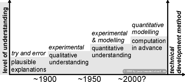
In table 1.2, a small collection of the milestones in the 200 years history of the arcing phenomenon is sketched. The arc discharge not only forms a basis for efficient discharge lamps, it is also an initiator for the development of plasma physics itself in the 1920's.
From discovery of a certain phenomenon (e.g. the use of metal halides for lighting purposes) to it's industrial use it can take more than 50 years and up to now, most practically important discharges cannot be computed in advance and thus may not be regarded as fully understood.
| Year | Contributor | Contribution |
| 1804 | Davy | carbon arc lamp |
| 1860 | Berthelot | electric arc methane to acetylene conversion |
| 1878 | Siemens | arc melting |
| 1890 | Moissant, Heroult | arc furnaces |
| 1901 | Marconi | arc radio transmitter |
| 1902 | Ayrton | monograph The electric arc [8] |
| 1905 | Birkeland, Schönherr | nitrogen fixation |
| 1911 | Steinmetz | principle of metal halide arc lamps |
| 1920 | Eggert, Saha | equilibrium composition in plasmas |
| 1923 | Compton | low pressure sodium lamp |
| 1930 | Pirani | 300 lm/W low pressure sodium lamp |
| 1933 | welding with carbon arcs | |
| 1935 | Elenbaas | high pressure mercury lamp |
| 1950 | Maecker | segmented arc for fundamental research |
| 1951 | inductrial plasma torches | |
| 1960 | USAF/NASA | multi MW wind tunnels for space reentry simulation |
| 1962 | commercial metal halide arc lamps | |
| 1963 | Schmidt | high pressure sodium lamps |
| 1965 | Paton | transferred arc plasmatron for stainless steel |
| 1977 | Liu | multidimensional model of the arc column |
| 1981 | Hsu | 1st attempt of a 2-D pLTE model for the arc column |
| 1984 | arc synthesis of fullerenes | |
| 1987 | Fischer | 1st 2-D plasma electrode model for high pressure lamps |
| 1988 | Palacin | 2-D model of the xenon short arc lamp column |
| 1989 | Tsai, Kou | column model with boundary fitted coordinates |
| 1990 | Delalondre | integrated 2-D column-cathode model |
| 1991 | low power high pressure mercury discharge car headlights | |
| 1995 | plasma- and cathode surface temperature measurements | |
| for the tungsten inert gas (TIG) welding arc are state of the art | ||
| 1997 | 2-D plasma-electrode models including convection | |
| are available for a number of discharge configurations | ||
| 1998 | commercial ultra high pressure (UHP)-mercury lamp (200bar) |
|
|
 |
Concluding from this long lasting history of the subject, every fifty years, there was a qualitative advance in the overall development paradigma (see figure 1.1). This work is dedicated to the actual change from trial & error supported by a first quantitative understanding to a computation of specific discharge features in advance.
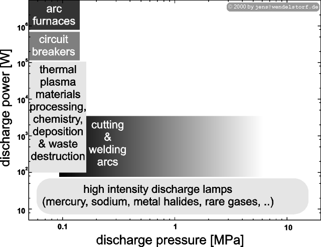
As demonstrated in figure 1.2, discharge powers range from a few W to several MW and discharge pressures are atmospheric in most cases. For lighting and (underwater) materials processing purposes, hyperbaric applications became more and more important in the last decades.
This work is dedicated to the computation and quantitative understanding of arc discharges. As a first step, the models will be applicable to stationary discharges showing cylindrical symmetry:
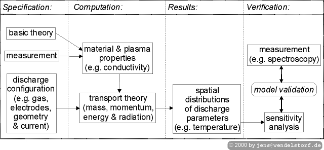
The common meaning of ab initio modelling is computation based on first principles and fundamental constants. The practical definition used for this work is sketched in figure 1.3:
An ab initio model is based on fundamental physics and any material, gas- or plasma property determined by a discharge configuration independent method. The model should not contain any parameter or input value which has to be fitted to experimental discharge data for every individual configuration under investigation. A practical ab initio model should allow for the computation of important discharge characteristics with an accuracy better than experimental error or sufficient for automatic optimization of discharge configurations.
The underlying motivation for model development with such high accuracy is the extrapolation capability these models should have. Additionally the strong nonlinear character of the arc discharge implies a need for relative high computation accuracy. The model validation by quantitative comparison with experimental data has to be supplemented by a sensitivity analysis: Some experimental quanitities are rather insensitive to changes in the arc configuration (e.g. doubling the current often implies only a few percent change in plasma temperature), while other are easy to determine (e.g. voltage-current characteristics) and also sensitive to important nonlinearity effects like mode transitions.
Sensitivity analysis has to be undertaken within all fields important for the development of the models and their validation:
One of the most important experience from modelling such systems can be summarized in one sentence:
The validity of the physical description of the system can be justified a posteriori (afterwards), but not a priori (in advance).
Another is the importance of a sensitivity analysis in order to obtain information about the role of a specific input parameter (e.g. electrode work function) on the overall or local discharge behaviour.
The modelling approach is therefore relying on the comparison with selected reproduceable experimental data of known accuracy. The answers of this validation and sensitivity analysis are not always positive:
The model will enhance the understanding of the arc phenomenon itself, but the overall objective is quantitative prediction of specific discharge configurations. Some sort of understanding of such complex systems can be obtained by many different plausible explanations or models with internal fit parameters. But these will fail if new discharge configurations are to be computed in advance.
| Chapter 1: | Introduction. |
| Chapter 2: | Conceptual framework for modelling electric arc discharges. |
| Chapter 3: | Physics of the electric arc discharge: |
| · Plasma column. · Electrodes. · Electrode layers. | |
| Chapter 4: | Plasma properties and transport coefficients. |
| Chapter 5: | Modelling results, validation and sensitivity analysis. |
| Chapter 6: | Summary, outlook and conclusions. |
Mathematical or physical modelling conventionally consists of a derivation of the equations describing the system and then solving them. This requires making all assumptions and approximations in advance. As the systems under investigation become more complex, this procedure becomes inapplicable in terms of effort and due to the nonlinearity of nature. Initially made assumptions need to be controlled afterwards and the modelling work becomes an iterative process itself.
Most of all important arc phenomena occur as an emerging result of the interaction of different physical processes and discharge regions. The accurate modelling of the individual parts of the discharge is a prerequisite, but the iterative linkage of these models is of the same importance.
As sketched in table 1.3, the overall modelling approach is discussed first in chapter 2. After sectioning the discharge into regions governed by different physical processes, the global iteration algorithms needed for the complete discharge description are presented. Within chapter 3, the physical models of the plasma column, the electrodes and the boundary layers are presented. The computation of the basic plasma properties and transport coefficients is summarized in chapter 4.
In chapter 5, the model proves its ability to reproduce all major discharge features. Initially, an easy computable arc configuration is selected, and the detailed results available from the modelling data are provided. Additionally, the impact and origin of the flow pattern formation are discussed. For this model lamp, the general arc behaviour is computed for a large range of external parameters. The rest of the chapter is dedicated to the validation of the model by comparison with available experimental data.
The last chapter (6) gives a summary of the achievements, it applications and the possible future enhancements of the model.
|
 |
The objective of this chapter is to develop the concept for an ab initio model of the overall thermal plasma gas discharge behaviour. As sketched in figure 2.1, there are at least three physically different regions:
Looking at the details of these regions, one realizes even finer structures, e.g. the boundary layer split into a space charge sheath and ionisation nonequilibrium presheath.
As a conclusion, the overall electric discharge system can not be described by a unified mathematical model, or such a model will be useless and untreatable. One has to realize a hierarchy of physical processes occuring in different regions, at different scales and with different relevance to specific features of the discharge. The electric arc is an arrangement of parts, so intricate as to be hard to understand or deal with - a complex system. Its behaviour emerges from a self organization of its parts.
For this reason, we have to look at the general behaviour and modelling tasks for general complex systems first, as provided in the next section. Within this framework, in section 2.2 the arc discharge is identified to show the behaviour of a Complex Adaptive System.
The specific modelling approaches for the individual arc regions are discussed in section 2.3. Here, we also provide the algorithms required to link physically and numerically different models without loosing their individual modelling accuracy. This and alternative approaches are discussed in section 2.3, followed by a summary of the whole chapter.
The overall target is not to develop a model of all possible discharge situations, but to develop a framework which may be regarded as sufficient for some simple arc configurations and open for further improvements. We treat the arc discharge as a dissipative complex system and we will get a comprehensive and simple picture of some discharges together with the identification of new complex phemomena relevant to others ¼ (just another iteration towards the impossible complete model).
This section is an adaption of the arc discharge relevant material of an introduction provided by Badii and Politi [9]:
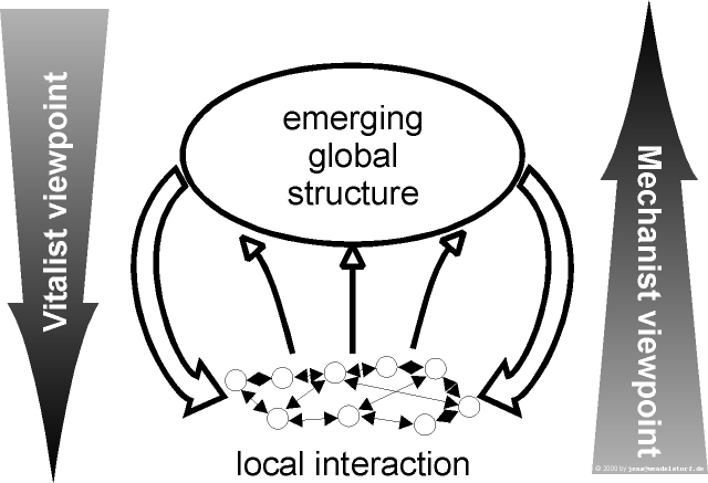
Research on complex systems means searching for general patterns in a number of very distinctive systems. Characterizing complexity in a quantitative way is also a vast and rapidly developing field. In general, complexity is not just another phenomenon, it may be regarded as another approach, contradictionary to the reductionist approach currently used in most areas of science (figure 2.2):
Whenever substantial disagreement is found between theory and experiment, the system has been observed with an increased resolution in the search for its elementary constituents. Matter has been split into molecules, atoms, nucleons, quarks, thus reducing reality to the assembly of a huge number of bricks, mediated by only three fundamental forces: nuclear, electro-weak and gravitational interactions.
The discovery that everything can be traced back to such a small number of different types of particles and dynamical laws is certainly gratifying. Can one thereby say, however, that one understands the origin of the arc discharge? Well, in principle, yes. One has just to fix the appropriate initial conditions for each of the elementary particles and insert them into the dynamical equations to determine the solution. Without the need of giving realistic numbers, this undertaking evidently appears utterly vain, at least because of the immense size of the problem. An even more fundamental objection to this attitude is that a real understanding implies the achievement of a synthesis from the observed data, with the elimination of information about variables that are irrelevant for the sufficient description of the phenomenon. For example, the equilibrium state of a gas is accurately specified by the values of only three macroscopic observables (pressure, volume and temperature), linked by a closed equation. The gas is viewed as a collection of essentially independent subregions, where the internal degrees of freedom can be safely neglected. The change of descriptive level, from the microscopic to the macroscopic, allows recognition of the inherent simplicity of this system.
These examples introduce two fundamental problems concerning physical modelling: the practical feasibility of predictions, given the dynamical rules, and the relevance of a minute compilation of the systems features.
In fact, as the study of nonlinear systems has revealed, arbitrarily small uncertainties about the initial conditions are exponentially amplified in time in the presence of deterministic chaos (as in the case of a fluid). This phenomenon may already occur in a system specified by three variables only.
The resulting limitation on the power of predictions is not to be attributed to the inability of the observer but arises from an intrinsic property of the system. In section 2.2, as an example, cathode phenomena in low pressure arc dicharges are identified to show such a behaviour.
Nature provides plenty of patterns in which coherent macroscopic structures develop at various scales and do not exhibit elementary interconnections. They immediately suggest seeking a compact description of the spatio-temporal dynamics based on the relationships among macroscopic elements rather than lingering on their inner structure. In a word, it is useful and possible to condense information.
Similar structures evidently arise in different contexts, which indicates that universal rules are possibly hidden behind the evolution of the diverse systems that one tries to comprehend. Many systems can be characterized by a hierarchy of structures over a range of scales. The most strong evidence of this phenomenon comes from the ubiquity of fractals (Mandelbrot, [86]), objects exhibiting nearly scale-invariant geometrical features which may be nowhere differentiable.
Hierarchical structures appear to be a general characteristic of nature. The difficulty of obtaining a concise description may arise from fuzziness of the subsystems, which prevents a univocal separation of scales, or from substantial differences in the interactions at different levels of modelling.
The concept of complexity is closely related to that of understanding, in so far as the latter is based upon the accuracy of model descriptions of the system obtained using a condensed information about it. Hence, a theory of complexity could be viewed as a theory of modelling, encompassing various reduction schemes (elimination or aggregation of variables, separation of weak from strong couplings, averaging over subsystems), evaluating their efficiency and, possibly, suggesting novel representations of natural phenomena. It must provide, at the same time, a definition of complexity and a set of tools for analysing it: that is, a system is not complex by some abstract criteria but because it is intrinsically hard to model, no matter which mathematical means are used. When defining complexity, three fundamental points ought to be considered:
After observing a new phenomenon, research initially attempts to find a quantitative measure for it. For complexity this is historically strongly related to discrete mathematics, coding and compression theory. Details may be found in the literature [9,110]. For our discharge modelling context, a specific meaning of the complexity measures is proposed as follows:
In the long term, the historical development of discharge models is clearly attracted towards descriptions with balanced complexity. In the short term, the development follows the path of least resistance, where increasing logical depth is simple and increasing sophistication is most difficult.
Before affordable high performance computers emerge in the 1980'ties, the development was focused on the mathematical description of specific physical processes relevant for specific arc configurations or regions. Obtaining numerical solutions was possible for highly simplified models only. Nowadays, special care has to be taken, when using measured quantities (like plasma conductivity) obtained using oversimplified discharge models.
 |
We speak of self-generated complexity whenever the (infinite) iteration of a few basic rules causes the emergence of structures having features which are not shared by the rules themselves. Simple examples of this scenario are represented by various types of symmetry breaking (superconductors, heat convection) and long-ranged correlations (phase transitions, cellular automata). The relevance of these phenomena and their universal properties discovered by statistical mechanical methods indicate self-generation as the most promising and meaningful paradigm for the study of complexity. It must be remarked, however, that the concept of self-generation is both too ample and too loosely defined to be transformed into a practical study or classification tool.
In any case, two extreme situations may occur: the model consists either of a large automaton, specified by many parameters, which achieves the goal in a short time, or of a small one which must operate for a long time. Consequently, the complexity of the pattern is often visualized either through the size of the former automaton or through the computing time needed by the latter.
Another aspect of the problem emerges, namely, that complexity is associated with the disagreement between model and object rather than with the size of the former. This, in turn, calls for the role of a subject (the observer) in determining the complexity itself through its ability to infer an appropriate model. Of course, a system look: complex as long as no accurate description has been found for it.
These considerations and the limited domain of applicability of all existing complexity measures strongly suggest that there cannot be a unique indicator of complexity, in the same way as entropy characterizes disorder, but that one needs a set of tools from various disciplines (e.g. plasma physics and computer science) and - of course - a significant amount of manpower and computer capacity. As a result, complexity is seen through an open-ended sequence of models and may be expressed by numbers or, possibly, by functions. Indeed, it would be contradictory if the complexity function, which must be able to appraise so many diverse objects, were not itself complex!
As sketched in figure 2.2, the global structure of a system is not unidirectional determined by the local interaction of its parts. The global structure may change local interactions. The objective of this work is not to change the viewpoint from reductionism (escape into detail) to holism (ignore the detail), but to apply both approaches as they are two sides of the same medal.
The electric arc discharge is driven by an external supply of electrical energy and permanently exporting heat and radiation to its environment. The plasma electrode system is far from thermodynamic equilibrium and exporting entropy. The discharge process is irreversible and can become chaotic. The distribution of the hot spots across the electrode surface or the discharge itself can show a fractal nature [45]. As shown in the next chapter, the effecive number of degrees of freedom can be reduced by exploiting its hierarchic structure. Such far-from-equilibrium systems manifest self-organization (synergetics). There are mathematical concepts for analysing time series data or nonequilibrium phase transitions by analytical methods [60]. In this work, there will be no attempt to extend these concepts to an only numerically treatable hierarchical system like thermal plasma gas discharges. An analytical treatment of the emerging discharge properties and thus the application of existing synergetic concepts is assumed to be possible by changing the type of the model from ab initio to heuristic.
A complex adaptive or self organizing system is not a mathematically well defined object. The arc discharge simply gets this characterization by another complex adaptive system - the human researcher investigating it. By accepting the complex details and their emerging properties, an increased understanding will finally allow the reader to characterize the arc as a less complex system.
 |
Now, we are prepared to realize the different levels of complexity appearing within the parameter range of high intensity gas discharges. This will enable us to define the arc systems predictable by actual modelling concepts (section 2.3) and possible extensions for the future.
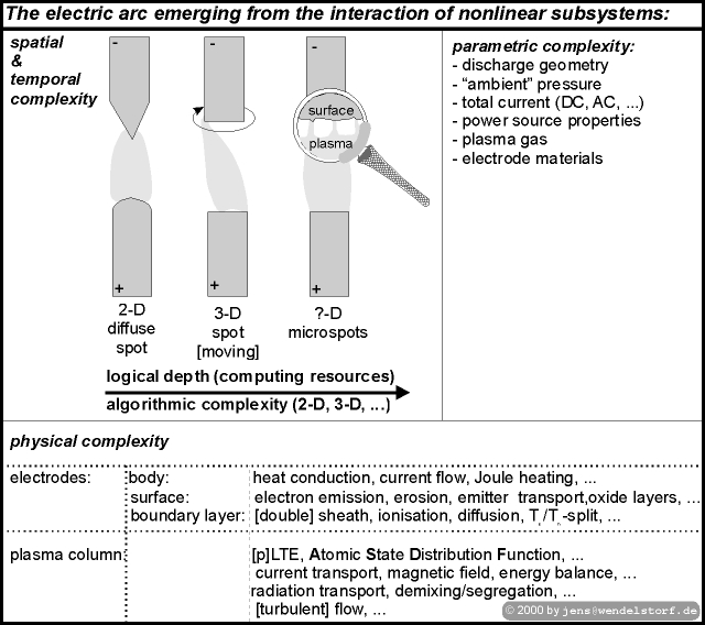
In figure 2.3, the different levels of complexity emerging in high intensity gas discharges are sketched. The physical details and models for them are discussed in chapter 3, here we discuss the three major spatial and temporal appearences of the overall discharge:
As a rule of thumb, the arc reacts on harder burning conditions with increased spatial and temporal complexity. The prediction of optimum burning conditions allowing for stationary cylindrical symmetric discharges is one of the objectives of this work.
A physical self consistent decription of the overall discharges (as described in chapter 3) needs to be based on a numerical solution concept, which is realistic in terms of development and computing time (algorithmic complexity and logical depth).
Modern methods of scientific computing have to be evaluated with respect to availability, costs and numerical effort. For electric arc modelling, the plasma is described as a conducting fluid. Mainly the concepts of Computational Fluid Dynamics (CFD) have to be applied. Because of its tremendous complexity and the amount of practical experiences needed for an understanding of such concepts, the following section can provide a summary only. Understanding will require at least the knowlegde of the basic concepts as described in standard textbooks [98,46,5,133].
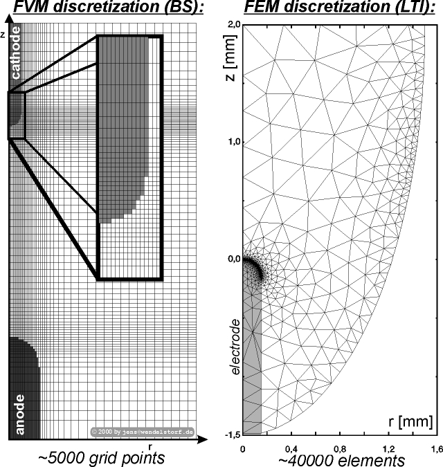 |
Regarding the numerical solution of the mathematical plasma electrode model, two different approaches are currently in use:
In their current implementation (BS: this work, LTI: [128,50]), both concepts have their specific drawbacks.
The orthogonal structured grid of the BS concept wastes a lot of grid volumes because the refinement depends only on the r and z coordinate. A solution adaptive refinement is implemented for the finite volume method by commercial CFD-codes (unstructured grids). The present approach was selected in order to limit code development time to a few years and because of the straightforward fluid flow implematation as described by Patankar [98]. Similar numerical concepts were implemented at CNRS/ENSCP in France [37], CSIRO in Australia [132,82], at UMN/ME in the USA [64,67] and several other groups.
The finite element arc modelling approach (LTI) is described in detail by Wiesman [128]. There is no inclusion of fluid flow phenomena in this implementation. The major drawback is not a numerical one, it is a result of the physical model used by the LTI approach. The neglection of one dimensional sheath effects and the description of the non equilibrium electrode layers by a 2D model implies the requirement for a very fine numerical mesh near the electrodes (see figure 2.4). The mesh elements scale down to a nanometer scale leading to a very large number of finite elements.
Both implementations (LTI and BS) may be regarded as less professional than commercial CFD/FEM software packages, but they allow for the prediction of electric arc behaviour, while commercial packages actually do not support this application.
In the future, easy to use and efficient arc modelling should be based on such commercial tools. The problem of these large codes is the unavailablity of the sources and their algorithmic complexity (more than 105¼106 lines of code compared to the several 104 lines developed at LTI and BS). For the development of the basic technology, the test and evaluation of new physical concepts and in order to have development times of only several man years, only concepts like those realized by this work and the groups cited above, are realistic. The following section will provide a summary of the general numerical concept for electrode plasma linkage (transfer function) developed within this work.
The orthogonal FVM discretization used for this work was selected for a maximum efficiency in code development time. This work is focussing on the investigation of physically self consistent and accurate cathode and anode layer models within the framework of a self consistent calculation of the overall arc discharge including convection effects.
The basic algorithm for solving coupled fluid flow and heat transport
problems by the finite volume method is perfectly described by Patankar
[98]. The early implementations of this approach for
an overall arc electrode model by a so-called conjugate heat
transport method can be found in the literature [82,132].
The solution of the 2D plasma equations (electric potential,
flow- and temperature-fields) as well as the heat (and current)
transport inside the electrodes can directly follow the
Patankar approach. His method solves a system of equations of the
type
| (2.1) |
| physical quantity | F | GF | Source SF |
| mass | 1 | 0 | 0 |
| axial momentum | u | m | - [(¶p)/(¶z)] + [(¶)/(¶z)] ( m[(¶u)/(¶z)] ) + 1/r [(¶)/(¶r)] ( mr [(¶v)/(¶z)] ) + jr BQ |
| radial momentum | v | m | - [(¶p)/(¶r)] + [(¶)/(¶z)] ( m[(¶u)/(¶r)] ) + 1/r [(¶)/(¶r)] ( mr [(¶v)/(¶r)] ) - m[(2 v)/(r2)] - jz BQ |
| energy | h | [(k)/(cp)] | [(jr2 + jz2)/(s)] - SR + 5/2 [(kb)/(cp e)] ( jz [(¶h)/(¶z)] + jr [(¶h)/(¶r)] ) |
| electric potential | F | s | 0 |
 |
 |
 |
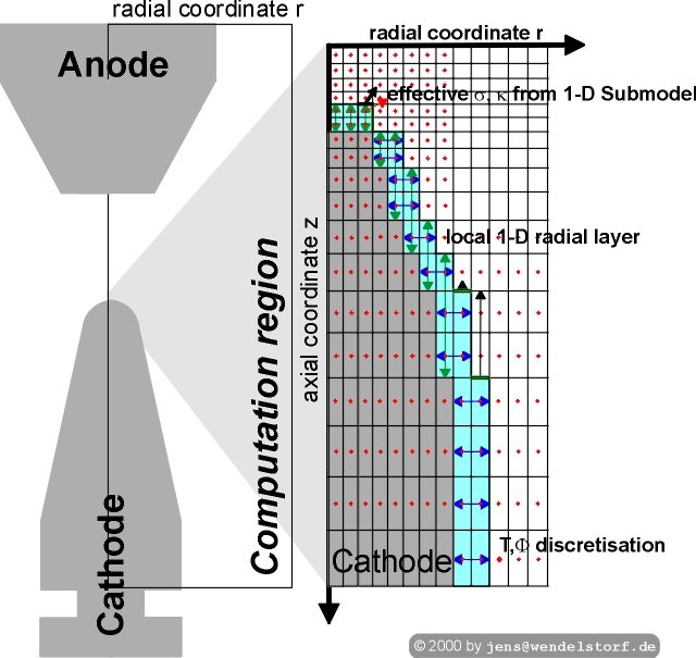
The major problem of the numerical concept is the development of a physically realistic and treatable boundary layer algorithm. In front of the electrodes, sheath effects occur (see chapter 3) and these are very difficult to implement into a 2D model. Because the size of the nonequilibrium layer is only about 10 mm (or even a few nanometers if the space charge layer is regarded as the boundary layer only), it can be treated as a 1D-layer forming a skin in front of the electrodes.
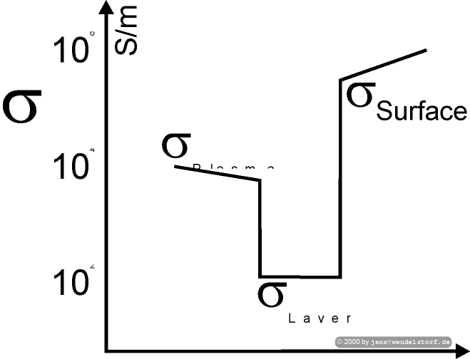
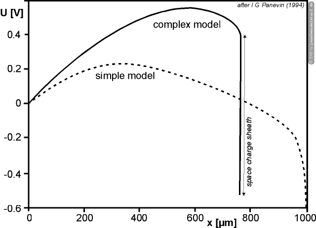
The finite volumes in front of the electrodes (resulting from the 2D meshing) require special attention. A numerically stable approach is to use a 1D layer model for the calculation of the effective electric and heat conductivity (figure 2.5). The result is a non smooth electric conductivity at the plasma electrode interface (figure 2.6). Negative anode sheath voltages (as resulting from the model described in the next chapter), will give even negative electric conductivities and can imply some numerical problems.
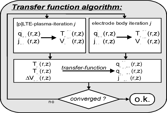
The effective conductivity approach works fine for some high current atmospheric argon arcs (see section 5.3.6), but it is not very realistic. Therefore the problem was generalized and found to be a special case of a general iterative scheme for the calculation of related boundary conditions for multidimensional regions linked by surfaces with additional physical processes to be modelled. This so called transfer function approach (figure 2.7) is very general and may also be used for other application areas or numerical schemes.
It is straightforward to get solutions for partial differential equations defined on multidimensional regions with well defined boundary conditions. Thus the electrode plasma system has to be divided into the 2D arc plasma and 2D electrode solid regions. The boundary conditions used for the 2D solutions are heat flux and voltage or current density. The layer between these regions is regarded as a black box transferring actual plasma and solid surface parameters to new boundary condition values for the next iteration step. As a result, the multidimensional regions are linked by a general scheme allowing for an implementation independent of a specific physical model of the processes inside the layer. It is a local concept allowing for a variation of the layer parameters and boundary conditions along the electrode surfaces. Regarding the plasma and solid heat balances, it simply transfers current values of the local plasma and surface temperatures to new heat flux boundary conditions.
As a matter of fact, electric arc discharges are not homogenous physical systems allowing for a description by a single set of equations. The internal boundaries between regions of different physical provenience and the long range interaction of the discharge parts form a self-organizing complex system. In the next chapter, the physical processes governing the individual regions will be described by mathematical modelling. The numerical linkage of the regions is sketched in this chapter. Finally the software implementation of this concept will deliver a computer model allowing to predict most of the characteristic features of the electric arc discharge. Through the emergence of more and more complex structures resulting from specific operating conditions and depending on discharge pressure, electrode geometry and discharge medium, the real arc may be still regarded as unpredictable for a randomly choosen configuration. But the remainder of this work will show the predicablitiy of a large class of discharge parameters: the stationary, radial-symmetric electric arc.
|
The overall aim of this chapter is to develop a numerically treatable ab initio model for a (large) class of thermal plasma gas discharges. Such electric discharges are also called electric arcs. Within the variety of gas discharges, the electric arc is defined by the following typical behaviour:
An introductionary discussion of the different types of arc discharges can be found in the literature [102,47]. Not all of them are treatable by the model described in this chapter or even any ab initio model to be developed in the near future. The model does not attempt to describe non-stationary multi-cathode-spot discharges (like vacuum arcs). Nevertheless, it can deliver the physical basis for future attempts to predict alternating current (AC) arcs used for lighting or welding.
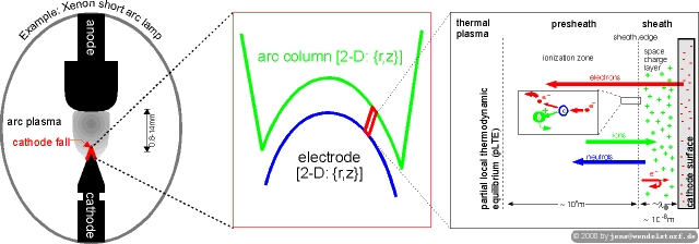 |
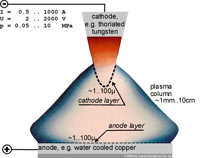
As sketched in figure 3.1, a typical arc discharge consists of a (highly luminous) plasma column linked to the electrodes by small (skin like) non equilibrium layers. The basic arc behaviour observed experimentally and discussed in the following sections will be predictable by the quantitative ab initio model developed in this chapter.
In order to obtain numerical solutions for the model developed within this chapter, the arc discharge has to be stationary and cylindrical symmetric. Most practical applications require such stable burning conditions which are realized by the following means:
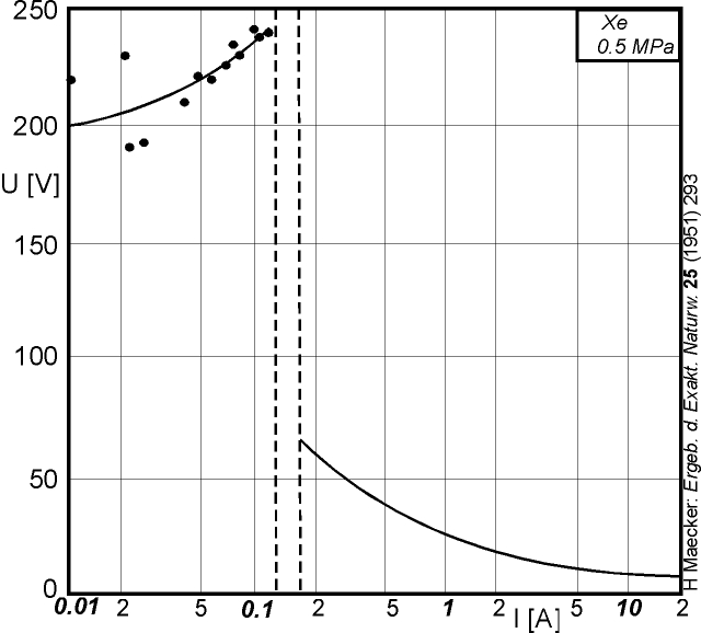 |
As shown in figure 3.2, the arc discharge is distinguished from the glow discharge by much lower voltages at higher current. The transition from glow to arc is in general non-smooth.
The current voltage characteristics of the arc is generally falling. Above a certain current (about 10 times the glow to arc transition current), the variation of the cathode fall is rather small. The anode fall voltage is nearly constant with current. The following model will allow for the calculation of all these voltage variations.
 |
 |
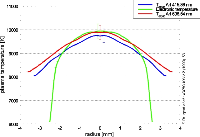
As shown in figure 3.3, the temperature profile in the column of (long) arc discharges is almost parabolic. Deviations of electron and heavy particles temperatures can be located (at least) in the arc fringes.
The electric field in the column of arc discharges is much lower than in glow discharges. This is due to the different ionization mechanisms. In the kinetic regime of the glow discharge plasma, the electric field must deliver electron energy up to the region of the ionization energy (Eion), while in the equilibrium arc discharge, the ionisation is due to the high energy tail of the electron energy distribution function, thus the electric field must only deliver electron energy of kbTe << Eion.
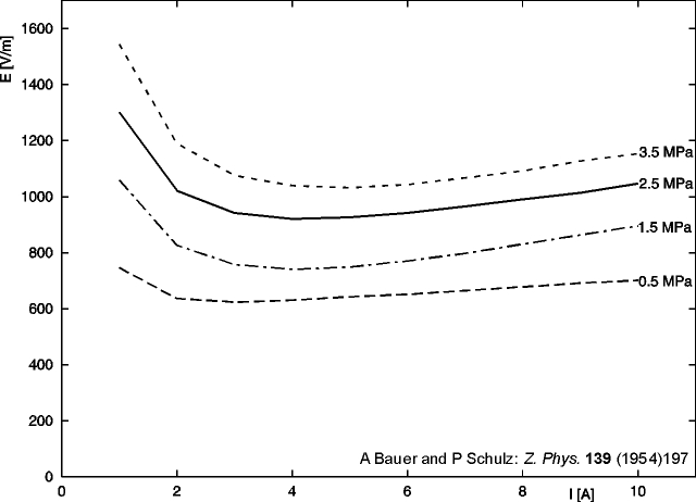
As shown in figure 3.4, the electric field in the center of the arc discharge increases with total discharge pressure (the mean free path to gain energy from the electric field decreases with increasing pressure) and the total current (heat loss by conduction, radiation and convection).
Glow discharges need a high cathode voltage drop, because the electrode is not at thermionic emission temperatures. The ions are accelerated in the cathode fall in order to provide an electron current sustained by secondary emission from the cathode surface.
The cathode voltage drop of the arc discharge is much smaller and its task is to heat the cathode surface to thermionic emission temperatures and to accellerate the emitted electrons for gaining energy needed for ionization within the near cathode plasma layer. Below a certain saturation current, the cathode fall voltage strongly depends on total arc current and decreases with increasing pressure.
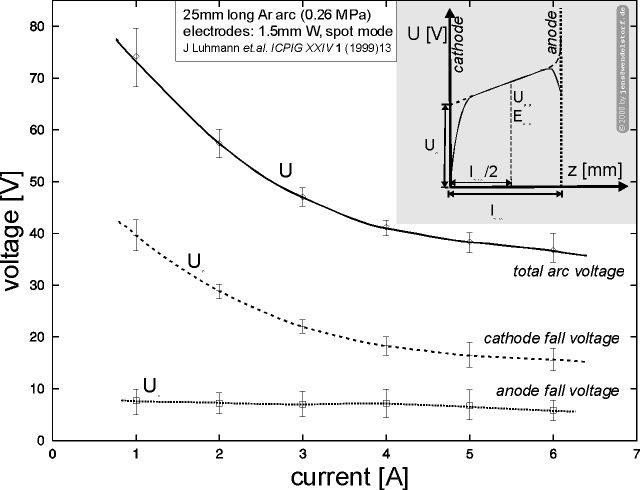
As an example, the strong current dependencies of the arc voltage, cathode- and anode fall voltages for a low current non LTE arc are plotted in figure 3.5. It can be seen, how the cathode heating required to reach thermionic emission temperatures is provided by the increasing fall voltage (located in the space charge layer) for total arc currents below 10A.
 |
Analogous to the situation at the cathode, the anode attachment can be diffuse, i.e. the current is spread over a relatively large area at a density of about 105¼7 A/m2. The energy flux densities are not very high compared to the spot mode and the material erosion is small as long as the evaporation temperature of the anode material is not reached.
If the increasing current is forced to occupy the edges or the anode surface structure is non-homogenous, the current density can increase locally by several orders of magnitude forming a single or numerous small hot spots.
Again, directly in front of the anode surface, a small space charge layer develops. If there is no need to supply additional energy for sustaining the electron current, i.e. the current density is below the electron saturation current density of the undisturbed column plasma, the fall voltage becomes negative.
In the case the anode surface area is smaller than the cross section of the column, there is also a plasma constriction near the anode resulting in an additional geometric fall voltage.
In most cases, the anode fall voltage does not vary appreciably with total discharge current (see figure 3.5).
In order to reproduce the basic features summarized above and to get accurate modelling software, at least the following physical phenomena have to be included in the discharge model:
As elaborated in the following sections, there are different models for different regions of the arc plasma. Very thin (skin like) non equilibrium layers in front of the electrodes are of special importance for the existence and formation of the arc itself. At least one of these layers, the space charge sheath, is small enough to be treated one-dimensional. Summarizing the results, the overall arc discharge model will consist of three sub-models linked by an iterative procedure:
Within the iteration algorithm, the data of the plasma and electrode surface is transferred to new boundary conditions for the next iteration cycle. The concept is thus called transfer function approach (see section 2.4). This approach can be implemented into the numerical simulation software independently of the specific details of the layer (1-D) or plasma/electrode (2-D) modelling and independent of the numerical procedures to be used for the 2-D regions (like finite volume or finite element methods).
The electrodes are heated within a small current-carrying
area, the so-called hot spot.
This heat load is dissipated by conduction and thermal
radiation of the surface. These losses and sources are boundary conditions
for the heat conduction equation to be solved within the electrodes:
|
 |
 |
 |
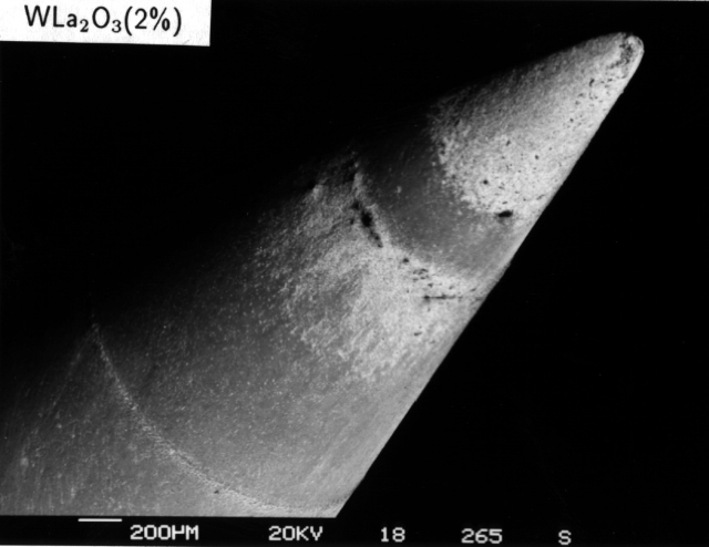
A typical welding cathode tip is shown in figure 3.6. The active (electron emitting area) is easy to identify, because the electrode surface is influenced by the high heat loads during arcing. Because electron emission workfunction is one of the most important electrode material parameters, real electrodes are often doped with low workfunction materials. As a consequence, surface and bulk diffusion of the emitter material [112] becomes important for the overall discharge behaviour and cathode lifetimes. Such non homogenous surface states imply spacially non uniform thermal radiation emissivities and work functions. In principle, the local radiation emissivity and electron emission work function therefore depends on local temperature and electrode composition. For a detailed investigation of the cathode surface structures and processes see [111].
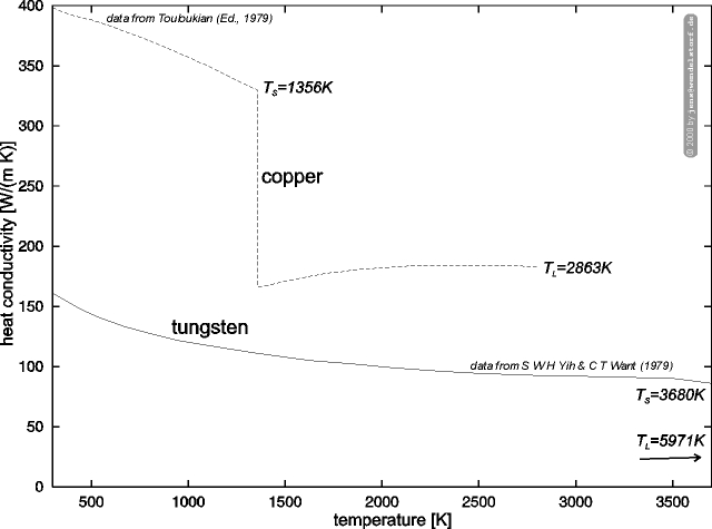
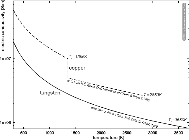
The heat and electric conductivity of typical electrode materials are plotted in figure 3.7. They are several orders of magnitude larger than the plasma conductivities. As a conclusion, current transport within the electrodes is not important for the overall discharge behaviour, while electrode geometry and heat conductivity significantly influences the hot spot formation at the cathode and thus the cathode fall voltage.
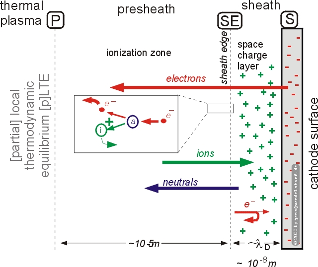 |
As discussed above and sketched in figure 3.8, the transition from the electron emitting cathode surface to a plasma in (partial) LTE can be further divided into a space charge layer (sheath) and an ionization layer (presheath). The interface between the thermal plasma and the presheath is associated with the subscript P, physical quantities at the sheath-presheath interface will be identified by the subscript SE, surface quantities by the subscript S. The sheath and presheath sublayers and their linkage are described in the following sections.
The local electron emission of the cathode surface depends on the local
surface temperature TS and the material property
work function F. It is given by
the Richardson emission formula [106]:
|
|
| material | F[eV] | AR [106 A/(K2 m2)] | Tmelt [K] |
| Re | 4.74 | 7.2 | 3453 |
| C | 4.53 | 0.6 | 3823 |
| Ta | 4.09 | 0.3 | 3269 |
| W (poly) | 4.52¼4.55 | 600 | 3653 |
| W (xxx) | 4.20¼6.0 | 600 | |
| W/ThO2/Th | 2.63 | 0.03 | |
| W/Ba | 2.66 | 1 | |
| W/La | 2.72 | 0.08 |
 |
For practical applications, the influence of the surface electric field ES on
electron emission is given by the Schottky correction formula (in eV)
[4]:
|
The work functions of some non refractive cathode materials used for high intensity arc discharges are summarized in table 3.1. The F and AR values in this table where determined experimentally (best fit to the Richardson equation). There seems to be a noticeable variation of AR. The values provided for doped tungsten materials are estimated and may also depend on the surface state of the electrode and the local surface concentration of the dopand.
Secondary electron emission by the impinging ion current ji is given by jSEE = gi ·ji where gi = 0.01¼0.3. It can be neglected for most arc discharge configurations. For low pressure discharges, gi becomes important. For argon with tungsten cathodes a value of 0.07 can be estimated [100].
In the case of high surface electric fields and cathode hot spot current densities, the emission current has to be calculated by the full thermo-field emission theory (see figure 3.9 and [99]).
The strong temperature and work function dependence of the emission current density determines the cathode hot spot temperature and may result in a bifurkation of the cathode hot spot system: Choosing optimum cathode geometry and a reasonable large discharge current, the arc contricts to a diffuse hot spot with current densities of 106 ¼108 A/m2 and several hundred microns in diameter (diffuse mode).
If the cathode is cooled by external means or by geometrical design, the hot spot may constrict below a critical current density and field electron emission becomes increasingly important (spot mode).
For the discharge the space charge layer (sheath) has the following functions:
The detailed potential and electric field distribution within the sheath is not relevant to the hot spot formation or overall discharge behaviour. The most important quantity, the voltage drop accross the layer US, is calculated by the energy balance at the sheath edge in section 3.3.3.
For the calculation of the electric field at the surface a simplified
model is used. In the case of a collision-free space charge sheath
(lia >> lDebye), the Poisson equation for the sheath
can be solved analytically for the electric field strength
at the cathode surface (see [84,125]):
|
|
|
For the overall current balance, the electron back diffusion
current is calculated by
|
|
As known since the beginning of the century [117],
one of the main purpose of the space charge layer is to
accelerate the emission electrons in order to
sustain the ionization within the presheath.
Approximately, the energy needed is given by the ion current
density at the sheath edge times the ionization energy
ji,SE ·Eion / e .
Within this estimate, the sheath voltage drop is given by
|
Benilov and Marotta [15] formulated a more accurate electron energy balance at the sheath edge which is used for this work:
There are two sources, the flux of energy brought into the layer by the emitted electrons accelerated in the space charge sheath jRS/e·(2 kbTS + eUS) and the work of the electric field over the electrons inside the layer calculated from the mean presheath electron current to [`(je,PS)] ·UPS, where UPS is the voltage drop accross the presheath. In the following the electron temperature Te means the electron temperature at the sheath edge.
The energy losses at the sheath edge are coming from the
electron back diffusion current leaving the presheath
for the sheath je,back / e·(2 kbTe+ eUS)
and the electron current leaving to the bulk plasma
jtot ·(5/2 + DeT) kbTe/ e
and the losses due to inelastic collisions required to sustain
the ion current ji / e·Eion.
Together with the current continuity condition, the following
equation system has to be solved for the current density
jtot and the space charge sheath voltage drop
US:
| |||||||||||||||||||||||||||||
For single charged ions, using DeT » 0.7 and
[`(je,PS)] = 1/2 (jtot + jRS - je,back),
the space charge layer voltage drop can be calculated for a given
ion current densitiy jion, emission current density
jRS and electron back diffusion current density
je,back, sheath edge electron temperature
Te and presheath voltage drop UPS
| |||||||||||||||||||||
A detailed one-dimensional model of the cathode layer was developed by Rethfeld and Wendelstorf [105] based on the work of Hoffert and Lien [62] also continued by Hsu and Pfender [66,64]. The presheath was identified as a stiff boundary value problem. The spatial variation of the plasma parameters can be adapted to almost every set of plasma and sheath boundary conditions.
For modelling the overall cathode hot spot self consistently,
only two parameters are important: the presheath potential drop
and the sheath edge ion current density.
First, the actual ion current ji
at the sheath edge can be calculated from the local current density
in the plasma jP, the electron emission current density
jRS and the electron back diffusion current je,b
|
|
|
| (3.3) |
The cathode layer model sketched above allows for the
calculation of all discharge relevant data without prior
knowledge of the detailed spatial variation of the
physical quantities in the presheath.
For controlling the physical validity
of the results, the presheath voltage drop can be
computed by the model of Benilov and Marotta
[15]. The presheath voltage drop is again calculated from
equation 3.3, but the sheath edge
electron density is calculated by a presheath model to
|
|
|
 |
The local net heating or cooling of the cathode surface
is given by a summation over all possible contributions
| (3.4) |
| ||||||||||||||||||||||||||||||||||||||||||||||||||||||||||||||||
|
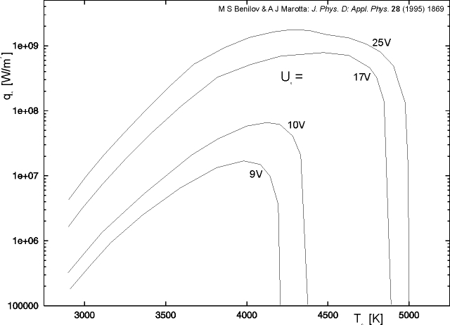
Within the cathode hot spot, qS is mainly given by ion heating balanced by emission cooling. The typical behaviour of this net energy flux density for different values of the sheath voltage drop is plotted in figure 3.10. From these plots, one can estimate the upper limit for the cathode hot spot temperature that is possible for a specific work function of the cathode material: 3630¼4610K for thoriated tungsten (F = 2.7eV) and 4340¼4905K for pure tungsten (F = 4.5eV) [43].
While the boundary conditions for the cathode surface are determined by equation 3.4, the electron energy balance of the plasma in front of the cathode surface is dominated by the Joule heating term and thus the major boundary condition is coming from the calculation of the local layer current density (equation 3.1).
Additionally, the following source term is included into
the energy balance within the cathode layer:
|
|
 |
Analogous to the cathode layer, the anode layer is divided
into a sheath and a presheath structure. The distribution
of the electric potential within this system is a bit
different to the one at the cathode.
As sketched in figure 3.11, the voltage drop
of the space charge layer is negative.
Assuming the anode is not emitting electrons, the current transport
is mainly due to the plasma electrons diffusing to the anode surface
against the (negative) space charge voltage drop
(the nomenclature is the same as for the cathode):
|
The voltage drop US is about several volts (3-8V) because the electron saturation current (US = 0) is above the usual current densities in the plasma.
As can be seen from figure 3.11, there must be a
location in the layer, where the electric field is zero. At this
position, the
electric current is only diffusive
(see also section 3.5.3):
|
Assuming a linearly descending ne(x), the sheath edge electron density becomes
|
|
Finally, the local net heating of the anode surface
is analogous to the cathode given by
| (3.6) |
| ||||||||||||||||||||||||||||||||||
The surface energy balance within the hot spot region of the anode is dominated by condensation of the current carrying electrons at the surface (qS,e,back).
Compared to the cathode layer model in section 3.3, this anode layer model is rather crude. For enhancement, there may be the need to perform a detailed local 1-D calculation instead of the pure analytical model used here.
Additionally, the role of energetic photons (UV resonance radiation, see also [35]) in the cathode and anode layers is currently not included into any self-consistent model, but can change the ionization balance in the presheath. The models used in this section does not require a detailed calculation of the presheath properties.
Electric arcs are rather complex entities because of their spatial inhomogenities and the amount of plasma physics necessary for a description of the discharge. While low pressure discharges require a more or less kinetic treatment, because at least the electron distribution function is non-Maxwellian, the thermal plasma of the arc can be treated by a multi-fluid approach. Additionally, the full multi-fluid theory [24] can be simplified to a one-fluid treatment regarding flow phenomena and a coupled two-fluid model regarding energy transport.
While the layer physics presented in the preceeding sections, provide the boundary conditions for the thermal arc plasma, the multidimensional description of this region (often called the arc column, but also valid for the near electrode plasma regions) is provided in the following subsections.
The thermal arc plasma is treated as a quasineutral (ne = ni) conducting fluid. Except for the energy balance, the electrons and heavy particles are treated as a single fluid.
| (3.8) |
| (3.9) |
From Newtons second law, the momentum equation is derived ([97] and [18]):

The total time derivative is defined as usual1. The strain-rate tensor \sf p is described in [97]. For cylindrical coordinates, \sf p can be found in [18]. The dynamic viscosity h is the proportionality factor between momentum current and velocity gradient and is calculated and discussed in section 4.6. Natural convection forces become important for high pressure arc lamps or gas shielding effects occuring in welding applications.
Regarding momentum transport, the type of the flow is
determined by the viscosity h, velocity u and characteristic
dimension l of the problem. From these quantitites, a characteristic
dimensionless number can be derived, the Reynolds
number:
|
Heat is generated in the plasma by Joule heating and carried away by radiation (net radiation loss coefficient SR, section 4.9), conduction (heat conductivity l, section 4.7) and convection. The compression work [(v)\vec] · [(Ñ)\vec] p and viscous dissipation [(v)\vec]:\sf p can be neglected, because the Mach-Number is about 0.1 and Prandtl-Numbers2 Pr = cp h/l are small (0.03¼0.7). Because the total pressure in the discharge region is mainly constant, the energy balance is formulated in terms of the plasma enthalpy h and reads

(For the Joule heating term one can often find the
equivalent forms j2/s or sE2).
The heat flux is given by conduction, enthalpy transport by the
(current carrying) electrons and the diffusion-thermo
(Dufuor) effect from the (de)mixing of different plasma components
[44]:
| (3.10) |
For simple one gas component plasmas,
the Dufuor effect vanishes and for
numerical convenience, the temperature formulation is introduced
([(Ñ)\vec] h = cp [(Ñ)\vec] T):
|
Even for modelling discharge configurations showing negligible deviations from LTE, the electron enthalpy flow term 5 kb/ (2 e) [(j)\vec] ·Te becomes undefined near the cathode layer, where a temperature split (Te ¹ Th) takes place in every discharge situation and the LTE model has to fullfill boundary conditions at the electrode coming from the heavy particle / electrode surface interaction3, while the electrons are thermally isolated by the space charge layer voltage drop.
Typical for thermal plasmas is the phenomenon of temperature split at pressures
below 0.1 MPa, at temperatures below 9000K and near the electrodes. The electrons
become decoupled from the heavy particles.
For this reason, accurate modelling requires the electrons and the heavy
particles to be treaten as different fluids (two-fluid model).
The energy balance of the electrons becomes
| (3.11) |
| (3.12) |
Analogously, neglecting transport of ionization energy [75],
the enthalpy balance of the heavy particles becomes
| (3.13) |
|
The heat conductivity is discussed in section 4.7. Incidentally, one has to distinguish between the general (3D) formulation given above, the (published) 2-D equations and the equations really treated by the individual computer code.
For this work (chapter 5), the full set of the equations is solved (without the Dufuor term, because no complex gas mixtures are investigated).
Regardless the importance of hydrodynamic transport phenomena,
the arc is mainly an electrical phenomenon.
Taking into account that the plasma column is electrical neutral
(quasineutrality, rel » 0), the generalized Ohm's
law becomes [47,122]
| (3.14) |
Because of the numerical difficulties of using
this generalized Ohm's law and because diffusion current
contribute less than 10% to the total current density
(except near the anode), most authors
use the conventional Ohm law
|
| (3.15) |
| (3.16) |
Starting with Ampere's law
|
|
|
|
|
|
For this work, the plasma geometry is radial-symmetric and
the axial current density component jz
is much larger than the radial one jr.
The magnetic field is simply given by
[(B)\vec] = {0,0,Bq }.
Neglecting the displacement current and with mr » 1,
Ampere's law reduces to
|
| (3.17) |
In high pressure discharges, diffusion of charged particles is not free.
There is a strong coupling between the electrons and ions.
This phenomenon is called ambipolar diffusion.
For the electric arc, the corresponding
diffusity Damb is almost identical to
the ion-atom diffusity Dia (see section
4.5).
The additional equation to be solved within the
(2 or 3D) plasma region reads:
|
An alternative approach more applicable for
arcs producing large plasma jets or influenced
by external gas flow, is to model the
neutral atom balance equation
|
Some applications like plasma gas cutting result in turbulent plasma flows. The inclusion of turbulence into the arc column model is reviewed in [127] and not used or discussed here.
Applying the physical models of the discharge regions sketched above, means making a number of basic assumptions, which are well justified and accepted:
These assumptions are valid for most discharge situations not too far away from LTE. This physical model requires additional computation of the plasma composition and transport coefficients depending mainly on electron temperature, as described in the next chapter.
Finally, the model will allow predictions for the overall discharge behaviour and the detailed spatial distributions of the physical parameters like plasma and electrode temperature. Results for a number of typical applications are provided in chapter 5.
It is evident from the different physical processes governing the main arc plasma and the sheaths, that the discharge cannot be described by a single set of equations. For physical self consistence, a proper definition of the internal boundaries and an iterative linkage of the submodels is cruical - as provided by this and the preceeding chapter.
|
The composition, thermodynamic properties and transport coefficients of thermal plasmas strongly vary with temperature. Their calculation in local thermodynamic equilibrium (LTE, Te = Th) is based on the work of Hirschfelder, Curtis and Bird [61] using tabulated partition functions [42]. Significant efforts where dedicated to the transport theory foundations since the early work of Devoto [38]. Starting 1977 [70], non equilibrium effects within the partial LTE concept (pLTE, Te ¹ Th) were introduced [64,20].
Focussing the efforts on modelling the overall arc discharge, the results of these references were selected and applied on the basis of the current knowledge from major working groups. The approach is to focus on LTE dicharges, but to use the two-temperature model in order to identify parameter ranges, where identical electron and heavy particles temperature in the main arc plasma (column) is not a valid assumption.
An ab initio decription of arc discharges more far away from LTE requires a closer look to the excitation equilibria [121] and is regarded not to be within the range of current modelling resources.
As summarized below, the plasma composition and transport coefficients show a strong variation with electron temperature, while the effects of temperature split (Q = Te/Th) > 1 are relatively weak. This does not justify the use of LTE models for discharges not in LTE, because deviations of electron temperature from the heavy particles temperature will imply important variations of plasma parameters and transport coefficients through the Te dependencies. As an example, the LTE electric conductivity of an atmospheric argon plasma at 5000K is almost zero, but allowing for an electron temperature of 10000K will give a conductivity of 2000 S/m. Such temperature split effects are important for all electric arc discharges within a small layer in front of the electrodes, where LTE is almost impossible (except for some sodium vapour lamps) because the heavy particles equilibrate with the surface but the electrons are thermally isolated through a potential barrier (space charge sheath). Using a two temperature model will permit a self-consistent computation of this thermal boundary layer and enables the inclusion of electron enthalpy flow into the overall energy balance, because this term requires the electron temperature gradient, especially near the electrodes.
In the following sections, the plasma composition and thermodynamic properties are calculated (section 4.2) and the basic collision integrals are provided (section 4.3). These are needed to calculate the transport coefficients used within the macroscopic models discussed in chapter 3:
The foundation for the calculation of all plasma transport coefficients is the determination of the plasma composition as a function of electron temperature Te and heavy particles temperature Th. The particle densities of the individual components are determined by the condition of quasineutrality, Daltons law and the Saha-Eggert equations.
Deviations from electrical neutrality (space charges) will produce
high electric fields efficiently restoring electrical neutrality.
On macroscopic scales, the plasma is thus electrical neutral
(quasineutral). The electron density is equal to the sum of all
ion densities times their ionization state:
|
Real gas effects (virial corrections) can be neglected
within the temperature and pressure range of thermal plasmas
[23]. The total discharge pressure is described by the ideal gas law.
The summation of the
contributions from the individual plasma components gives:
|
At total discharge pressure levels above 10 MPa, the plasma becomes
non-ideal. For a weak non-ideality, the Debye pressure correction
can be introduced [55]
|
The ionization equilibrium of the plasma
is described by a system of Saha-Eggert equations [121,120]
|
The partition function Z is given by its translational, rotational,
vibrational and internal contributions:
|
|
|
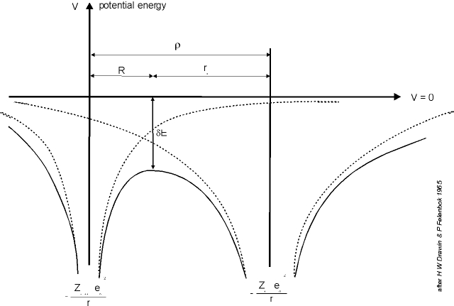 |
The exact energy levels of the ions and atoms within the plasma cannot be computed ab initio, thus the undisturbed energy levels of the free atoms and ions are used. The divergence of the partition function is avoided by a so called cut-off criterion (figure ) [56], allowing to calculate the lowering of the ionization energy:
|
| (4.1) |
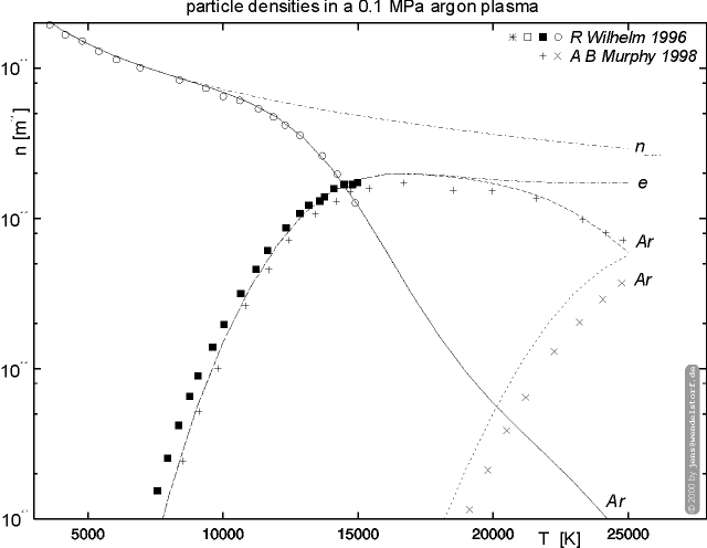 |
The calculated particle densities are in good agreement with the values published in the literature (figure 4.2). The cut-off criterion has significant effects on viscosity and reactive heat conductivity only [29,90].
|
 |
As shown in figure 4.3, the mass density is sensitive to the non equilibrium parameter Q = Te/Th. This is due to Daltons law. As the total particle number increases with the onset of ionization, the ideal gas scaling r ~ 1/T is not valid above the onset of ionization (e.g. above Te = 9000K for 0.1 MPa argon).
|
| |||||||||||||||||||||||||||||||||
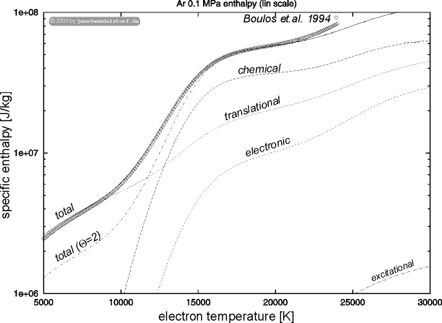 |
The high temperature enthalpy (figure 4.4) is dominated by chemical and translational enthalpy, while excitational enthalpy can be neglected.
| (4.2) |
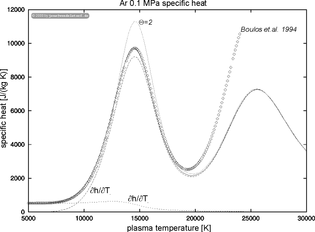 |
The temperature dependence of the specific heat reflects the different ionization levels within the plasma (figure 4.5).
The basic particle interactions (collisions) within the plasma
are modeled by the calculation of so-called collision integrals.
The interaction between the different particles within the
plasma (atoms, ions and electrons) can be described by
an interaction potential depending on the relative
(kinetic) energy of the collision partners. The calculations assume
binary instantanous collisions. Details are
described by Hirschfelder, Curtis and Bird [61].
The collision integral of the order (l,s) is defined by
[7]:
|
| |||||||||||||||
For a number of simple interaction potentials, the collision integrals are tabulated relative to the hard sphere values or given by analytic approximations. Otherwise, the collision integrals are computed by numerical integration. In the following subsections, the different collision categories are discussed.
Collisions between neutral particles are modeled
by a Lenard-Jones interaction potential
|
Compared to other estimates, the collison integrals for
temperatures above 1600K (for Argon) deviate by less than
20% (see table 4.2 and [76]).
This will give slightly wrong values
for the low temperature viscosity but has no remarkable
effects regarding electrical and heat conductivity.
For this interaction potential,
the collision integrals can be related to the
corresponding hard sphere values
|
Collisions between charged particles are modeled
using a screened Coulomb potential. The collision
integrals are tabulated [87,40].
Allowing for a deviation of about 15%,
an analytical approximation can be used [78]:
| ||||||||||||||||||||||||||||||||||||||||||||
Charge exchange collisions between ions and atoms can be modeled
by the heuristic interaction potential
|
These collisions dominate the collision integrals [`(Q)](l,*) for even l. For odd l, Devoto has computed some values for argon. A comparison with the even l charge-exchange collision integrals gives a scaling factor of 1/4 , avoiding the extensive calculations done by Devoto and without the requirement of detailed atomic data. Alternatively, a simple polarisation model (dipol interaction) can be used [130].
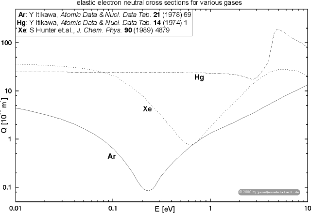
Electron atom collisions are highly affected by quantum mechanical matter wave inflection (Ramsauer effect). The cross sections can be measured [68] or calculated [3]. The collision integrals are calculated numerically using cross section data from the literature (see figure 4.6).
 |
| plasma gas: | Ar | Xe | Hg | Tl | I |
| Z [1] | 18 | 54 | 80 | 81 | 53 |
| m [u] | 39.948 | 131.29 | 200.59 | 204.383 | 126.904 |
| E* [eV] | 11.660 | 8.313 | 4.670 | ||
| Eion1 [eV] | 15.755 | 12.130 | 10.434 | 6.1083 | 10.44 |
| Eion2 [eV] | 27.626 | 27.626 | 18.761 | 20.428 | 19.0 |
| Eion3 [eV] | 40.911 | 40.911 | 34.21 | 29.83 | 31.4 |
| rLJ [10-10m] | 4.055 | 3.465 | 2.898 | 4.055 | 4.320 |
| tLJ [K] | 229 | 116 | 851 | 116 | 210.7 |
| Q0,CT [10-20m2] | 7.5 | 48 | 12 | 17 | 5.6 |
| aCT [1] | 0.13 | 0.14 | 0.11 | 0.12 | 0.16 |
| Qen(E) ref. | [101] | [51] | [94] | [94] | [108] |
| T[K] | Qe,Ar+ (1,1) | Q Ar,Ar (2,2) | QAr,Ar+(1,1) | QAr,Ar+(2,2) | Q e,Ar (1,1) | |||||
| Devoto | this work | Devoto | t.w. | Devoto | t.w. | Devoto | t.w. | Devoto | t.w. | |
| 5000 | 12200 | 11467 | 20.4 | 25.1 | 98.5 | 96 | 28.7 | 23 | 1.48 | 1.7 |
| 10000 | 1510 | 1281 | 17.6 | 22.7 | 87 | 89 | 23.2 | 21 | 3.46 | 3.5 |
| 20000 | 358 | 305 | 15 | 20.7 | 76.2 | 83 | 18.7 | 19.8 | 7.11 | 6.9 |
Using the simplifications discussed above and the fundamental data provided in table 4.1, reasonable agreement with the more detailed computations of Devoto where found (table 4.2). This gives a sufficient accuracy for a large number of plasma gases where the basic data needed is available, while more sophisticated calculations like those of Devoto will require unaffordable efforts or will be even impossible due to missing fundamental data.
The elastic energy exchange between electrons and heavy particles is computed by a mean collision frequency approach [17,31]:
|
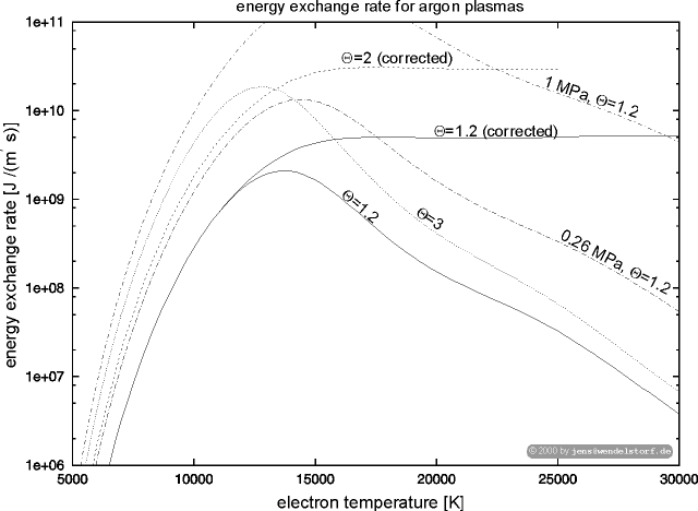 |
The energy exchange (see figure 4.7) between the electron fluid and the heavy particles drastically increases with pressure.
With increasing electron temperature, inelastic energy exchange between
electrons and heavy particles should be taken into account.
The detailed computation of this rate coefficient is
extremely difficult. The principal dependency is
|
The principal parameter dependencies of the diffusities
are [130]:
|
The binary diffusion coefficient of two plasma species is given by [61]:
|
|
|
Because macroscopic space charge formation is not possible (quasineutrality condition),
the flux of electrons and ions out of any region must be equal
(neglecting the net total current). This coupling avoids independent
diffusion of charged particles. The coupled diffusity is called
ambipolar diffusity and given by [79]:
|
Using the Einstein relation for the mobility and diffusity ratio
ma/Da = e/(kbT)
and the fact of much higher electron mobility
me >> mi, we get
|
For practical applications in high pressure discharges, the ambipolar diffusity is almost identical to the ion-atom diffusity Dia.
The proportionality factor between momentum current and
velocity gradient is called dynamic viscosity. The principal
dependence on plasma parameters is as follows [130]:
|
| (4.3) |
|
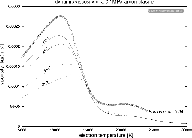 |
The electronic contribution is less than 2 % and thus neglected [23]. Due to this small influence of the electrons, viscosity decreases with increasing non-equilibrium parameter Q (figure 4.8). The difference of the calculated viscosity to that provided by Boulos [23] is due to different treatment of the atom-atom interaction.
Heat transport in thermal plasma gas discharges can be split
into an electron contribution le dominating the high
temperature regime and a heavy particles contribution lh
dominating the low temperature regime:
|
Using only the dominating translational heat conductivity, the principal
dependence on plasma parameters is as follows:
|
|
| ||||||||||||||||||||||||||||||||||||||||||||||||||||||||||||||||||||||||||||||||||||||||||||||||||||||||||||||||||||
The i = 2 ¼N summation is taken over all heavy particles.
The heavy particles heat conductivity is calculated from the
translational, reactive and internal contributions
|
Using the second approximation from [91], the
translational heat conductivity of a multicomponent plasma
is given by
|
| |||||||||||||||||||||||||||||||||||||||||||||||||||||||||||||||||||||||||||||||
Due to the variation of the excitation of the internal degrees of freedom of the plasma components with temperature, a corresponding heat conductivity can be defined [7]:
|
| |||||||||||||||||||||||
This contribution is at least one order of magnitude below translational and reactive heat conductivity and can be safely neglected.
Diffusive particle transport in a fluid with chemical reactions (like ionization and recombination) lead to the transport of chemical enthalpy. The corresponding heat conductivity is taken from [28,25]. Taking R chemical reactions (incl. ionization) into account, it is given by:
|
| |||||||||||||||||||||||||||||||||||||||||
 |
 |
As shown in figure 4.9, the total plasma heat conductivity le + lh is in reasonable agreement with literature data and not strongly affected by the non-equilibrium parameter Q. The heavy particles heat conductivity is strongly affected by the reactive peak due to the onset of ionization.
In high density plasmas with low ionization degree, the
electric conductivity is determined by electron mobility
and electron density, thus the principal dependencies are:
|
Here, the electric conductivity is calculated using the approximations of Devoto [39]:
|
| ||||||||||||||||||||||||||||||||||||||||||||||||||||||
 |
As an example, the temperature dependence of the electric conductivity is shown in figure 4.10. There is no significant Q-dependence and excellent agreement with literature data.
In general, the effective radiation emission is
computed by subtracting spectrally integrated emission
and absorption :
|
Because the numerical effort for a detailed treatment
of the radiation transport is tremendous [88],
an effective net radiation emission
coefficient as described by Lowke [81] is used for this work.
The net radiation loss function Srad(Te) was
computed at the University of Karlsruhe [119] by integration of the specific spectral radiation emissivity
el:
|
The following radiation emission mechanisms are taken into
account:
| |||||||||||||||
The line emission coefficient elbb denotes the radiated
power per solid angle, which stems from spontaneous radiative transition
between two discrete energy levels. In LTE it depends on the population
density of the upper level Ek, when the transition probability
Aki is known, and reads
|
|
The continuum radiation arises from recombination
(free-bound) and bremsstrahlung
(free-free) transitions and is usually
given in terms of hydrogen, with appropriate
correction factors, the so-called Bibermann
factors x. For a high-pressure plasma the contribution
of electron-atom encounters has
also to be taken into account, and the continuum
emission coefficient becomes
|
The terms can be calculated from [12]
| |||||||||||||||||||||||||||||||||||||||||||||||||||||||||||||||||||||||||||||||||||||||||||||
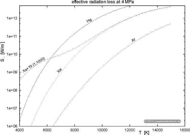 |
 |
In figure 4.11, the net radiation emission coefficients calculated in Karlsruhe are visualized. Doping the discharge medium with low ionization potential materials can have a strong effect on the radiative properties at lower temperatures. The radiation source strength at a specific plasma temperature linearly increases with pressure [11].
For the optical thick radiation an effective radiative heat conductivity can be calculated [6,88,129]. Recently, a full treatment of the radiation problem came into the range of treatable models [88].
For a number of applications, the thermal plasma is
not in ionization equilibrium. The ionization rate is proportional
to electron and atom density, recombination is mainly a three
particle reaction A+ + e + e ® A* + e. The net ionization
rate is defined to be
|
|
Following the detailed computation of the recombination
rate coefficient [16], one can use the following simple approximation
[62]:
|
| Tr. Coeff. | 100% Value | Qea | QCT | QCoul. | Qaa |
| s(T = 5kK) | 26 S/m | -0.9 | 0.0 | -0.1 | 0.0 |
| s(T = 7.5kK) | 940 S/m | -0.5 | 0.0 | -0.5 | 0.0 |
| s(T = 10kK) | 3390 S/m | -0.3 | 0.0 | -0.7 | 0.0 |
| k(T = 5kK) | 0.04 W/(m K) | 0.0 | 0.0 | 0.0 | -1.0 |
| k(T = 7.5kK) | 0.11 W/(m K) | -0.3 | 0.0 | -0.2 | -0.5 |
| k(T = 10kK) | 0.42 W/(m K) | -0.3 | -0.2 | -0.4 | -0.1 |
| n(T = 5kK) | 1.8·10-4 kg/(m s) | 0.0 | 0.0 | 0.0 | -1.0 |
| n(T = 7.5kK) | 2.3·10-4 kg/(m s) | 0.0 | 0.0 | 0.0 | -1.0 |
| n(T = 10kK) | 2.2·10-4 kg/(m s) | 0.0 | -0.2 | 0.0 | -0.8 |
| parameter | 100% Value | all Q's | Qea | Qia | Qee | Qaa |
| Varc | 11.8 V | 0.2 | 0.2 | ±0.02 | 0.1 | -0.1 |
| VC,el. | 8.0 V | 0.2 | 0.2 | ±0.03 | 0.2 | -0.3 |
| VA,el. | 2.7 V | 0.2 | 0.0 | ±0.01 | -0.1 | 0.3 |
| Ecol. | 882 V/m | 0.6 | 0.4 | ±0.01 | 0.1 | ±0.1 |
| Tcol. | 7444 K | 0.1 | 0.05 | 0.0 | 0.0 | 0.04 |
| TC,max. | 3306 K | 0.0 | 0.0 | 0.0 | 0.0 | 0.0 |
| vmax. | 0.5 m/s | 0.5 | 0.2 | ±0.02 | -0.02 | 0.6 |
| Srad,max. | 5.7·109 W/m3 | 1.8 | 1.2 | ±0.06 | 0.2 | -0.1 |
| rad. yield | 0.3 | 0.8 | 0.4 | ±0.03 | 0.1 | 0.3 |
The sensitivity gives the principal dependency of the transport coefficient or arc parameter
f on the cross section data Q:
|
For the transport coefficients, the sensitivity is trivial (table 4.3: They are proportional to 1/Q (s = -1). The electric conductivity depends on Qea for low ionization degrees and on QCoul, for higher ionization degrees. The total plasma heat conductivity depends on Qaa for low and on all Q's for high ionization degrees. Viscosity is dominated by atom-atom interaction (Qaa).
The influence of cross section data on the basic arc properties is shown in table 4.4. Decreasing or increasing the numerical values of the cross sections (e.g. by multiplication with 1.5), normaly changes most arc properties by less than 20%. The column electric field (and thus the arc voltage for longer arcs) more strongly depends on electron-atom interaction (Qea). Global arc parameters with strong temperature dependencies like the radiative properties show more significant changes with changing cross sections, especially the Ramsauer data (Qea) can have remarkable influences. Because the complex and nonlinear nature for the arc-electrode system, such sensitivities will also depend on the specific discharge situation and can be calculated only for small deviations from a given parameter set.
|
In the previous chapters, a self consistent physical model of the complete arc discharge was developed (chapter 3). The necessary plasma transport coefficients were computed (chapter 4), and the basis of the numerical calculation schemes was discussed (chapter 2).
This chapter will first show detailed results predicted for a simple (in terms of geometry and computing time) discharge configuration. This will give an impression of the discharge properties emerging from the interaction of the different physical processes discussed in chapter 3. The influence of the details of the physical model on the overall discharge behaviour will become evident from a physical sensitivity analysis.
By a variation of the fundamental arc parameters like current, gas, pressure and cathode properties, the model will prove its ability to reproduce all major discharge features. The discharge properties visualized for these parameter studies are mostly obtainable by experiment. Thus the results can be regarded as predictions of future measurements.
The experimental validation of the model will be discussed in further detail and some comparisons with existing measurement data will be presented.
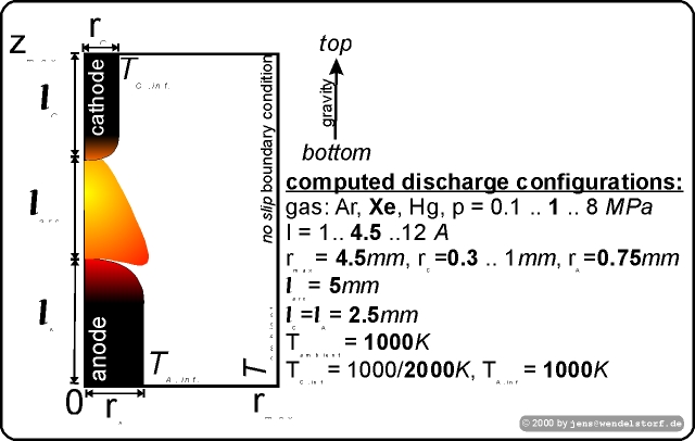 |
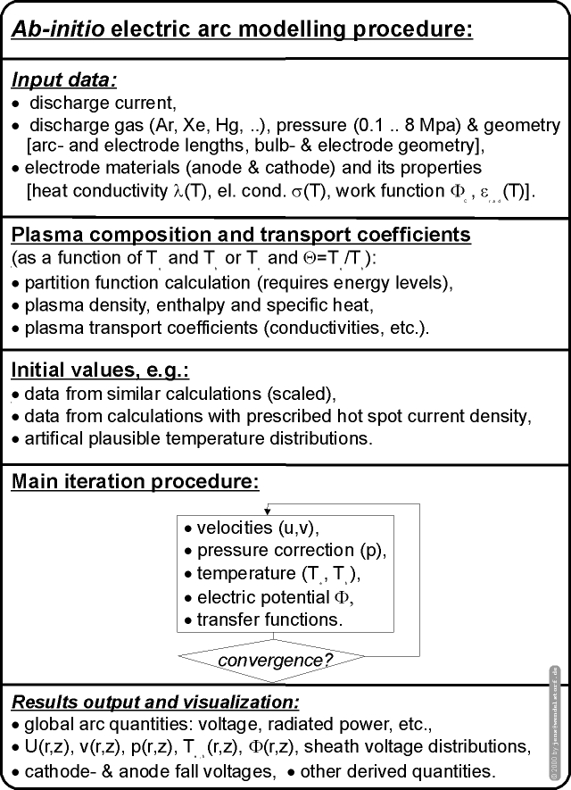 |
The computational effort (logical depth) of the numerical solution for the complete arc model is tremendous. It scales with the spatial dimensions of the discharge and the dimensions of the electrodes. Very high current densities within the cathode hot spot require numerical parameters (e.g. the virtual time step) far beyond the capability of current computers. The model lamp was therefore selected to be relatively small. Nevertheless, it can be realized experimentally and the results are very usefull for the understanding of a large and economically important class of thermal plasma gas discharges, the high pressure arc lamps, also called High Intensity Discharges.
In figure 5.1, the model lamp configuration is sketched and the fundamental parameters and boundary conditions are provided. If not otherwise stated, the numerical calculations include the following effects:
All these equations are solved within the iterative procedure scetched in figure 5.2). The geometry is always cylindrical, and the numerical grid is non equidistant with smaller finite volumes in front of the electrodes.
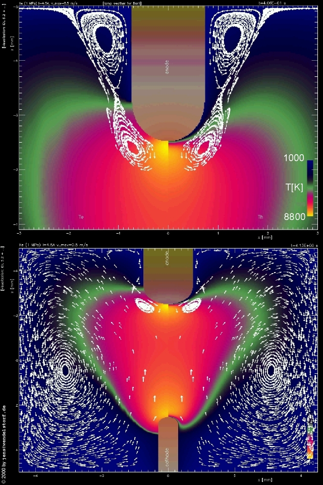 |
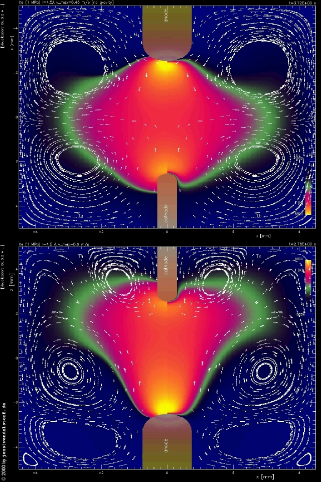 |
First of all, the spatial distribution of the plasma temperatures and the flow field within the discharge is visualized in figure 5.3. Regarding fluid flow, the driving forces within the model lamp are mainly natural convection (gravity) and the magnetic compression resulting from the high current densities near the cathode and anode hot spot. For a lamp burning vertically with the cathode at the bottom, convection is dominated by a flow vortex with the center in a torus around the arc. The magnetic forces due to the constriction of the arc current within the near anode plasma act against the cathode and the buoyant jet coming from the cathode at the bottom. As a result, a second vortex structure emerges around the anode (top of figure 5.3). Because of the high impact of convective heat transport, the arc temperature distribution follows the flow field. Finally, the temperature map looks like a reversed bulb. For this plasma gas (xenon) and discharge pressure level (1 MPa) and current (4.5A), the arc is mostly in LTE (Te = Th). Near the electrode surfaces, the electron temperture decouples from the heavy particles temperature. This thermal boundary layer results from the thermal isolation of the electron fluid due to sheath effects, while the heavy particles equilibrate with the electrode solid.
Reversing the burning position of the arc (figure 5.4, bottom), a similar temperature map results, but the cathode and anode exchange their roles. Due to the higher impact of the cathode jet now working against natural convection, the overall flow field is more complex. There are three major vortex structures emerging: The main vortex around the center of the discharge is smaller, and has two child vortices at the bottom. The vortex around the cathode at the top is larger and the overall flow field will be more sensitive to disturbances.
Neglecting buoyancy (gravity) effects, the impact of the flow field on the arc temperature map is smaller and a two vortex structure emerges (figure 5.4, top).
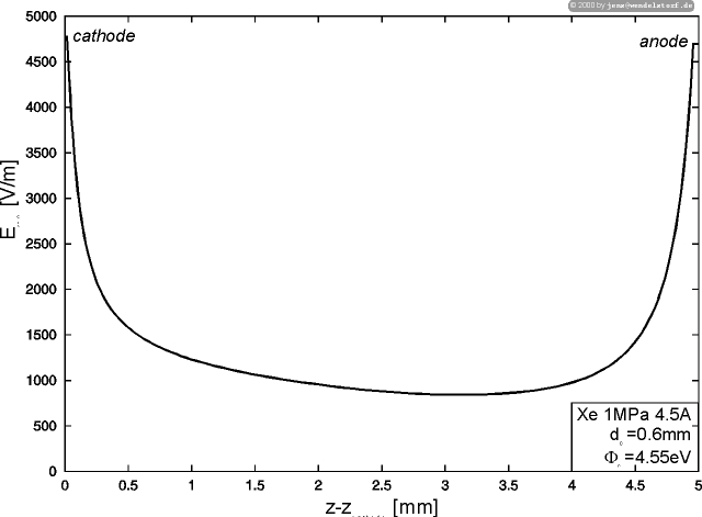 |
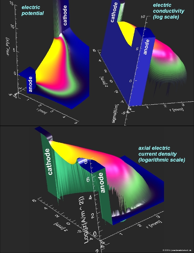 |
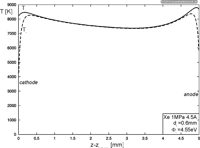 |
The spatial temperature and velocity distribution of the arc (figure 5.3) is mainly caused by the spatial distribution of the electrical quantities visualized in figure 5.6. The upper left picture shows the electric potential distribution within the arc electrode system. The main voltage drop is located in the space charge layer around the cathode surface. The anode sheath model used here, delivers a self consistent negative space charge layer voltage drop around the anode surface. This voltage drop is limiting the diffusive electron current from the plasma to the prescribed total current level and a current density level determined by the electric conductivity of the near anode plasma. The upper right picture gives an impression on the spatial distribution of the electric conductivity within the arc electrode system. Because the conductivity of the solid electrodes is several orders of magnitude larger than that of the thermal plasma, the conductivity drop gives rise to the important sheath effects included into the model. The picture at the bottom provides an impression of the current constriction within the cathode and anode hot spot. The resulting high electrical current densities lead to the magnetic compression forces driving the flow field within these areas.
The electric field strength on the arc axis is plotted in figure 5.5. Near the cathode and anode surface, the plasma constriction requires electric fields around 4500 V/m, while the electric field in the arc center is rather small (geometrical decompression in the column). In this region, the current carrying area is much larger (the sheath induced electric fields at the electrode surfaces are not visualized here).
The axial plasma temperature distribution (figure 5.7) allows to estimate the thickness of the thermal boundary layer near the electrodes, where non LTE effects occur. The high electrode hot spot current densities increase the ohmic heating of the plasma. As a result, the plasma temperature shows two maxima within the thermal boundary layers at the electrodes.
 |
The model does not use any prescribed boundary conditions at the cathode or anode surface. The net heat flux distribution at the electrode surfaces is emerging self consistently from the interaction of electron emission, plasma sheaths and constriction near the surface. As shown in figure 5.8, the energy balance within the cathode hot spot is determined by ion heating, electron emission cooling and heating due to the neutral gas temperature gradient.
 |
 |
The electrical current density at the cathode surface (figure 5.9) is given by the electron emission current density and the ion current coming from the presheath.
While the overall discharge model used here does not require a detailed model of the cathodic ionization layer (presheath), it is possible to compare the resulting ion current coming from the presheath with the results from the one dimensional model developed by Benilov and Marotta ([15], section 3.3.5). Figure 5.9 shows the excellent agreement of both modelling approaches.
As shown in figure 5.10, the major assumptions of the layer model (see section 3.6) agree with the mean free paths in the near cathode plasma.
 |
After discussing the spatial distribution of the basic physical arc properties, the modelling input parameters plasma gas, discharge pressure, total current, cathode diameter and electron work function will be varied.
The first and most important quantity of thermal plasma
gas discharges, the voltage current characteristic is shown
in figure 5.11. The high burning voltages
for very low currents can be identified with the increase
of the space charge layer sheath voltage with decreasing current.
The self consistent presheath voltage slightly increases with current,
while the cathode fall voltage defined by
| (5.1) |
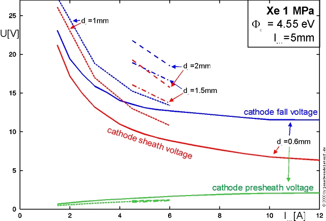 |
Larger cathode diameters increase the heat losses of the cathode and thus require higher sheath voltages to increase the energy of the impinging ions heating the cathode surface to thermionic emission temperatures (figure 5.12).
 |
Increasing pressure slightly enhances the layer and cathode fall voltages due to the smaller ionization degree of the plasma (figure 5.13). The larger increase in arc voltage with increasing pressure is caused by the larger electric fields required in the main arc core, because radiative, convective and conductive heat losses increase and electric conductivity decreases. At lower pressure levels, the cathode fall voltage can become larger than the arc voltage, because the anode fall voltage becomes negative.
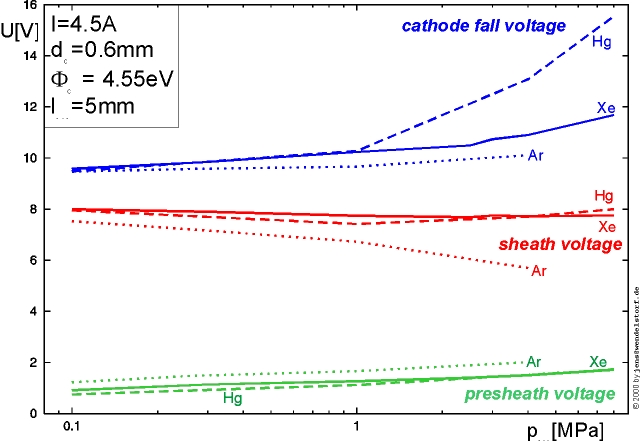 |
Varying pressure for different plasma gases (figure 5.14) shows how gases with low ionization energy like mercury require higher cathode fall voltages with increasing pressure, due to the increasing voltage drop in the near cathode plasma. Because above 1 MPa the argon plasma undergoes a transition from partial LTE to LTE in the arc column, the sheath voltage may even decrease with pressure,
 |
One of the main purposes of the space charge layer (sheath) is to accelerate the ions in order to gain energy for heating the cathode to thermionic emission temperatures. With decreasing cathode work function FC, the sheath voltage is thus also decreasing (figure 5.15).
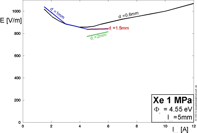 |
 |
The minimum electric field in the arc column (determined from its axial variation shown in figure 5.5) depends on current and pressure (see also figure 3.4). As shown in figure 5.16, the model is able to reproduce this fundamental arc property. The effect of the cathode properties like diameter dC is rather small. For most discharge configurations electrode effects on this quantity vanish with increasing arc length.
Higher discharge pressure levels increase the radiative, convective and conductive energy losses. To carry the prescribed arc current, the electric field in the arc column increases with pressure (figure 5.17). Due to the missing ramsauer minimum and its larger values, the electron-atom cross section causes much higher electric fields in mercury discharges than in xenon or argon.
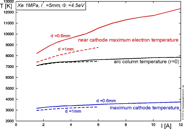 |
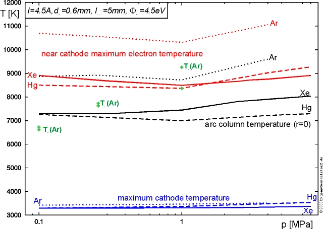 |
 |
In figure 5.18, the variation of the plasma and cathode hot spot temperatures with arc current is shown. The column temperature is slightly increasing due to a small variation of the energy balance in the arc center with increasing current. Its absolute value is mainly determined by the variation of electric conductivity with electron temperature. The near cathode maximum of the axial electron temperature distribution strongly depends on current (increasing current densities increase the joule heating term) and electrode properties like cathode diameter (figure 5.18) and work function (figure 5.20).
Depending on the ionization threshold temperature of the plasma gas, the plasma temperatures are larger for inert gases (figure 5.19). Additionally, for low current levels and pressures below 1 MPa, the argon arc is not in local thermal equilibrium (LTE). As shown in figure 5.19, with decreasing pressures an increasing gap between electron and heavy particles temperature in the argon arc column occurs.
The cathode hot spot surface temperature is not very sensitive to the discharge gas or pressure. It mainly depends on the cathode work function (figure 5.20) and the cathode geometry (figure 5.18). Due to the workfunction effect on the hot spot current density, the maximum electron temperature also increases with the cathode material work function.
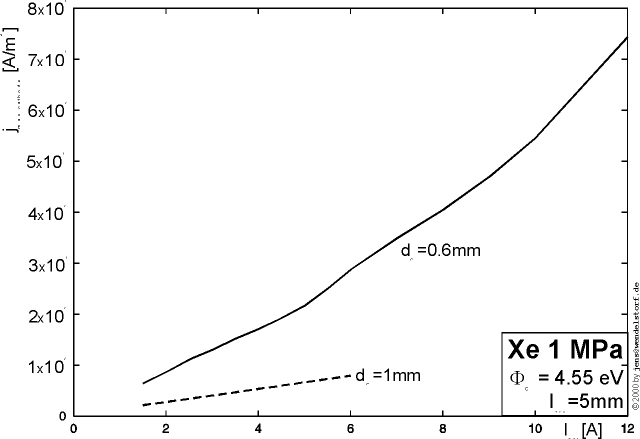 |
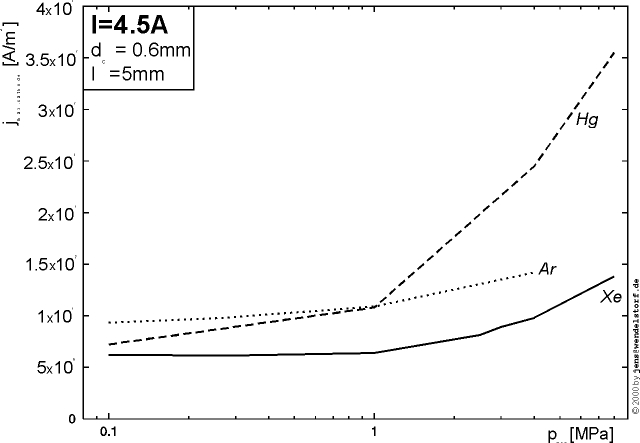 |
 |
All computations where carried out for a diffuse cathode hot spot. The electric current density on the cathode surface varies with position (figure 5.9) and its maximum value on the axis is plotted in figure 5.21, figure 5.22 and figure 5.23. Small cathode diameters introduce an additional constraint for the current density distribution, because the plasma has to follow the cathode curvature and the current density is strongly determined by the energy balance within the cathode. For small cathode diameters, the peak current density is thus strongly increasing with current, while for larger diameters the current density increase is much smaller (figure 5.21). A further increase in cathode diameter or very low currents will finally result in a change of the cathode attachment mode.
For atmospheric discharge pressures, the effect of the plasma gas and pressure on cathode peak current density is much smaller than for pressure levels above 1 MPa (figure 5.22). In such high pressure discharges, the effect of the higher electric field, required in the arc plasma to carry the prescribed current, gives also rise to increasing peak current densities.
Decreasing the cathode work function allows for lower cathode surface temperatures and a flattening of the current density distribution is energetically prefered. The peak current densities are thus smaller for smaller cathode work functions (figure 5.23).
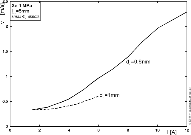 |
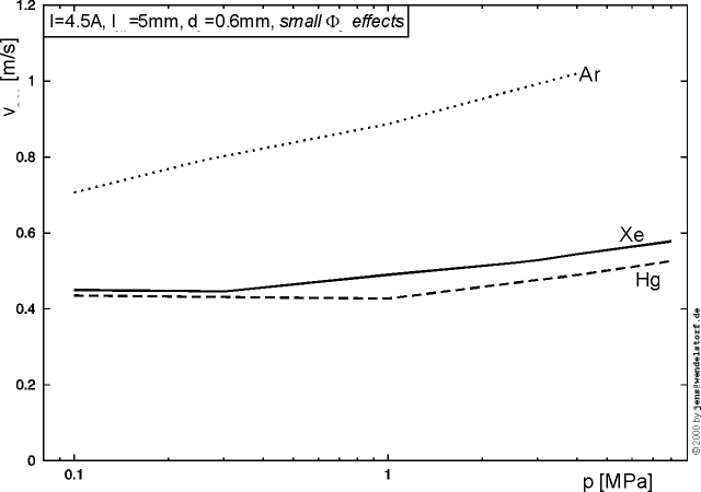 |
The maximum axial flow velocity is mainly determined by the magnetic compression in the cathode hot spot (cathode jet). As the peak current density increases with total current, the maximum velocity follows (figure 5.24).
There is also an increase with discharge pressure (figure 5.25), because additional natural convection forces accelerate the flow for this burning position of the arc (cathode at the bottom). The effect of the discharge gas on maximum flow velocity can be explained by the atomic weight of the gas particles.
 |
 |
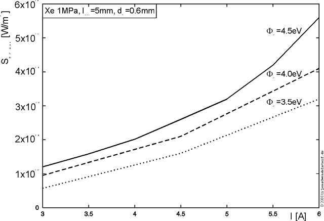 |
For lighting applications as well as for the spectroscopic determination of plasma temperatures, the maximum radiation intensity generated within the discharge is cruical. Because detailed radiation transport is not modeled here, only the maximum net radiation emission coefficient can be taken as a measure for this quantity. Due to the rather crude anode sheath model, the maximum net radiation emission coefficient calculated at the axial near cathode electron temperature maximum is provided as a measure of the radiation intensity properties of the discharge.
For small cathode diameters, the increase with arc current is rather strong (figure 5.26). This effect is again caused by the increasing current density (figure 5.21). The order of magnitude of the radiative intensity is first given by the radiative properties of the discharge gas and second by the discharge pressure (figure 5.27). The effect of cathode work function on the peak current density and thus maximum electron temperature can also be found in the increasing net radiation emission coefficient with increasing work function of the cathode material (figure 5.28).
 |
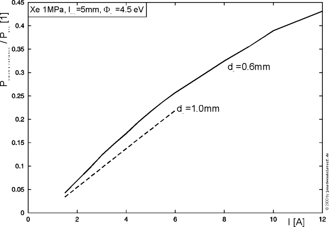 |
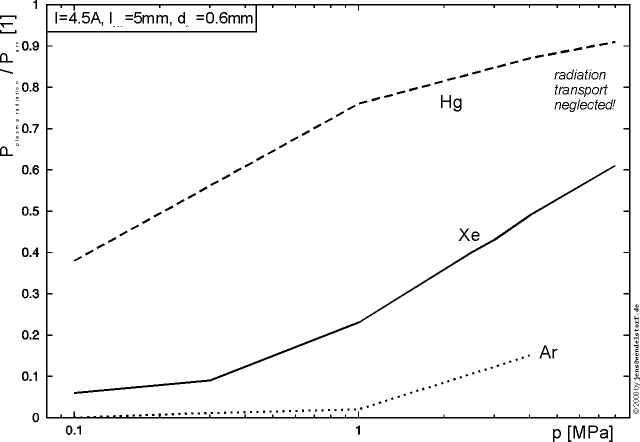 |
Because high pressure arc discharges are high performance sources of radiation, it is worth to look at the plasma radiation yield, i.e. the total power radiated by the plasma relative to the total power of the discharge (figure 5.29, figure 5.30 and figure 5.31). Due to the sharp increase in the net radiation emission coefficient with electron temperature, the radiation yield follows the dependencies of the maximum electron temperature and thus the peak electric current density in the cathode hot spot. It linearly increases with current (figure 5.29) and strongly depends on the radiative properties of the filling gas (figure 5.31). The increase of the radiation yield with decreasing work function shown in figure 5.29 can be explained by a change in the spatial distribution of the plasma temperature. A wider temperature distribution can provide a larger area at high electron temperature and thus higher radiation yields.
In reality, the high radiative yields of the mercury discharge at very high pressures (figure 5.31) are limited by radiation transport phenomena not included in the current model. For lamp fillings like mercury and discharge pressures above several atmospheres, a quantitative calculation at least requires an inclusion of a radiative heat conductivity into the model (see section 5.3.5).
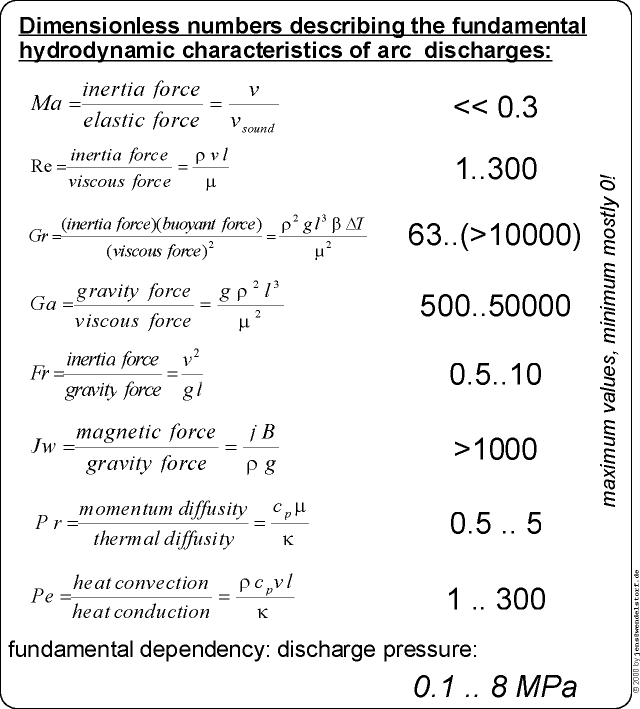 |
From figure 5.32 the importance of flow phenomena in general and of natural convection and magnetic compression in detail can be estimated. The Reynolds number is above unity but well below the critical values for turbulence. The plasma will show fully developed laminar flow. The Peclet number is always above unity, therefore one should not calculate thermal plasma gas discharges without taking fluid flow effects into account.
Nevertheless, the arc is mainly an electrical phenomenon, and the influence of the different physical effects has to be computed for every specific discharge situation. The validation of most physical approximations can not be done in advance.
| variant: | U | UC,PP | Emin | TC,max | Te,col | Te,C,max | SR,C | SR% | jC,max | vmax |
| 1. all 3 A | 13.6% | 12% | 3.7% | -2.8% | -1.4% | -5.2% | -54.1% | -37% | -34% | -28% |
| 2. all 4.5A | 11.4 | 9.9 | 819 | 3301 | 7402 | 8422 | 4·109 | 24% | 6·106 | 0.5 |
| 3. all 6 A | -2.4% | -3.2% | 4.2% | 2.1% | 1.6% | 5.1% | 103% | 28% | 44% | 45% |
| 4. fine grid | 1.5% | 0.9% | 2.8% | 0.6% | 0.5% | 0.5% | 11% | -0.9% | 17% | 3.4% |
| 5. no flow | -7.9% | -6.6% | -6.2% | -0.6% | -2.4% | -3.0% | -35% | 6.5% | -14% | - |
| 6. top down | -2.6% | -9.1% | 1.7% | -0.5% | 1.0% | -3.0% | -35% | 16% | -12% | 12% |
| 7. no gravity | -3.7% | -0.9% | -11% | -0.1% | -2.8% | -1.2% | -14% | 5.6% | -1.2% | -23% |
| 8. no [(j)\vec] ×[(B)\vec] | 1.0% | 0.4% | 3.3% | 0.1% | -0.1% | 0.0% | 2.7% | -1.6% | 2.2% | -52% |
| 9. " & td | -6.2% | -12% | 5.1% | -1% | 0.8% | -4.2% | -46% | 16% | -21% | -54% |
| 10. no [(j)\vec] [(Ñ)\vec] Te | 3.6% | 3.8% | 1.2% | 0.2% | 0.1% | 0.8% | 14% | -1.7% | 7.2% | -0.2% |
| 11. US = const. | 4.3% | 0.3% | 2.7% | 3.7% | 1.1% | 9.5% | 251% | -3.1% | 159% | 20% |
In table 5.1, the physical sensitivity matrix of the model discharge configuration is provided. The values of the second row are absolute quantities in SI-units, while all other values are given as the relative deviation to the second row.
U denotes the total arc voltage, UC,PP the cathode fall voltage (equation 5.1), Emin the minimum electric field in the arc column, TC,max the maximum cathode temperature, Te,col the plasma temperature in the center of the arc column, Te,C,max the maximum plasma temerature in front of the cathode, SR,C the maximum net radiation emission coefficient (see section 4.9), SR the amount of radiated power compared to the total arc power, jC,max the maximum current density at the cathode surface and vmax the maximum flow velocity in the discharge.
The table is based on calculations for the model arc configuration (Xe 1MPa, 4.5A, dC = 4.5mm, FC = 4.55eV) on a non equidistant grid of 48x96 finite volumes. It has to be interpreted as follows: The first and third rows show the variation of the basic arc parameters with total discharge current and the fourth row shows the relative deviation for calculations with a very fine numerical grid (144x288 finite volumes or more). In the following rows, the relative deviations obtained by switching off the different physical effects included into the discharge model are presented. Deviations smaller than the numerical error provided in row 4 are questionable and should be interpreted very carefully. The basic results of this physical sensitivity analysis are as follows:
As a conclusion, neglecting one of the different driving forces of the flow ([(j)\vec]×[(B)\vec] or gravity) can have larger effects on the results than neglection of flow phenomena at all. A quantitative computation of the radiative properties of high-pressure lamps strongly demands for the full inclusion of flow phenomena. For mercury, at pressures above 2 MPa, the radiation transport has also to be described in detail. Radial symmetric calculations are not possible for arcs burning horizontally. With increasing pressure, even discharges with cylindrical symmetry may develop three dimensional or turbulent flow patterns.
As a result of the basic parameter study and the physical sensitivity analysis presented above, a number of fundamental problems regarding the experimental validation of arc models must be taken into account:
In the following sections, a number of discharge configurations with available experimental data is presented and the modelling results are compared with experiment in order to obtain an overall model validation statement and a testimony for the individual physical descriptions of the arc regions.
 |
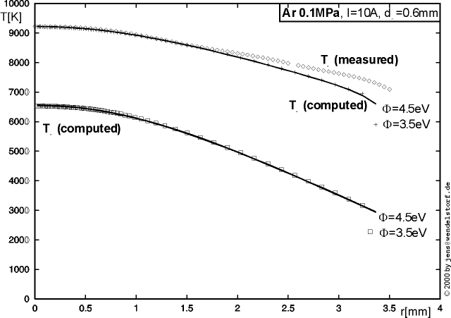 |
The experimental determination of the cathode fall voltage and plasma temperature map is difficult for high pressure discharges. It is more affordable and simple to perform measurements for argon discharges at or around the atmospheric pressure level. Especially at total currents below 50A, the arcs show very few radiation from the arc column and thus the electrode temperatures may be determined by thermography. It is also possible to determine the electron- and heavy particle temperatures as well as the electron density by spectroscopical methods.
As shown in figure 5.33, the computed temperature distribution of such low power atmospheric argon arcs is far away from LTE. The electron temperature level lies about 50% above the heavy particle temperature. These results demonstrate the ability of the model to describe non-LTE discharges. At current levels above 10A, there is excellent agreement between the measured arc temperatures and the modelling results (figure 5.34). Thus the model has proven its ability to calculate discharge situations not in LTE.
Nevertheless, a further decrease of the overall discharge current gives rise to another non LTE effect currently not implemented into the model: The deviation from Ohm's law (see section 3.5.3). At a current of 5A or less, the measured electrical field in the arc column is twice the electric field calculated by Ohm's law. As a result, there is a quantitative disagreement of the calculated temperatures (figure 5.35) and electron densities (figure 5.36).
Because the main purpose of the discharge is to heat the cathode surface to thermionic emission temperatures, the cathode fall voltage is dominated by the sheath voltage for such discharge configurations. Such a little impact of the electric field in the arc column on the cathode fall voltage results in an excellent agreement with the measurements (figure 5.37). Nevertheless, the model is not able to reproduce the overall burning voltage for discharges so far away from LTE. The computed and measured anode fall voltages do not vary with arc current, but their absolute values differ due to the very simple anode layer model and the large deviations from Ohm's law near the anode.
 |
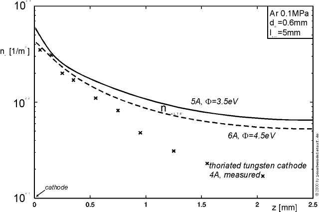 |
 |
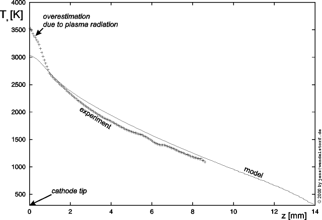 |
Some initial experimental data for 1 MPa xenon discharges at 1-6A are available. This section will provide a comparision with this data and a prediction of the values to be measured in the future.
The major problem of this discharge configuration is the instable arc observed experimentally and predicted by the failure of stationary calculations including fluid flow. All modelling results are therefore coming from computations without any convection effects.
The discharge geometry is that described in figure 5.1, with lC = lA = 14mm, rC = 0.3mm, rA = 0.75mm and larc = 20mm. The temperature boundary condition for the electrodes at z = 0 and z = zmax is 300K.
| I[A] | U[V] | UC[V] | US[V] | UPS[V] | E[V/m] | jC[A/m2] | TC[K] | PC,¥ [W] |
| 6.0 | 18.6 | 8.7 | 5.8 | 1.3 | 621 | 7.04·106 | 3356 | 5.7 |
| 4.5 | 18.6 | 8.9 | 6.2 | 1.2 | 612 | 5.03·106 | 3293 | 5.8 |
| 3.0 | 18.9 | 9.1 | 6.9 | 1.0 | 613 | 3.14·106 | 3205 | 5.8 |
| 1.5 | 20.9 | 9.8 | 8.3 | 0.7 | 666 | 1.40·106 | 3066 | 5.7 |
The calculated discharge parameters shown in table 5.2 are provided to give an approximate prediction of the values to be measured in the near future by Prof. Mentel's group at Bochum University [83]. Because of the neglection of fluid flow (as a result of the arc instability caused by the large arc length and tube diameter), and the uncertainty in the cathode work function5, the accuracy is only about 3V for the cathode fall voltage and about 100K for the cathode hot spot temperature. An additional error for the overall arc voltage may result from the simple anode layer model.
The comparison with initial experimental data for the cathode surface temperature distribution shows sufficient agreement (figure 5.38) - nevertheless the uncertainty in the cathode work function has to be taken into account.
This discharge configuration was defined for comparison of modelling results with experimental data. The calculated arc parameters show reasonable agreement with the first measurement values available. For a quantitative model validation, the discharge configuration has to be changed. Additional efforts are required to eliminate the principal errors induced by inaccurate input data like cross sections and work functions. As a conclusion, the quantitative validation of this or similar discharge models can be done only with respect to a specific quantity to be computed. Additionally, the validation has to be performed for a wide range of discharge pressures and currents.
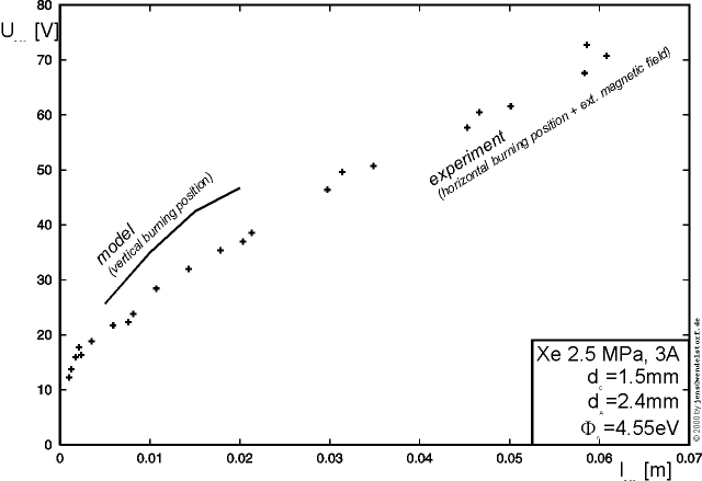 |
In 1954, Bauer and Schulz made detailed measurements of arc voltage, cathode fall and electric fields for horizontally burning high pressure xenon arcs [13]. This section is an attempt to calculate a similar discharge configuration, and to compare the results with the data from Bauer and Schulz.
As shown in figure 5.39, the experimental arc voltages are slightly below the computed ones. Before treating this fact as a problem of the model, one should take into account the external magnetic field and horizontal burning position Bauer and Schulz used for their experiments. The modelling results where obtained for the vertically burning arc configuration with the cathode at the bottom.
The calculated cathode fall is 23.6V for a discharge pressure of 2.5 MPa, while Bauer and Schulz measured 14V for 3.5MPa and 26V for 1.5MPa. The comparison gives evidence to the need for an exact reproduction of the experimental configuration by the model or vice versa. Additionally, the calculation of the cathode fall from the modelling results for only one arc length (equation 5.1) is justified for long wall stabilized arcs only.
Because of the large computing times needed, is was not possible to get modelling results for all discharge configurations used by Bauer and Schulz.
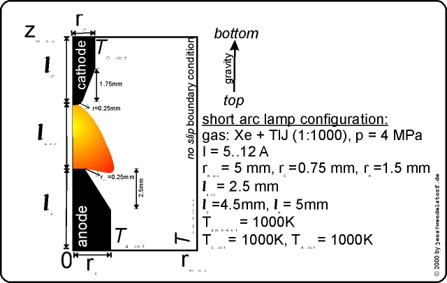 |
 |
 |
One of the direct application areas of the model are high pressure short arc lamps. The DC arc is burning in mercury and xenon at pressure levels between 5 and 80 atmospheres (0.5 to 8 MPa). The cathode is tipped, and the anode is relatively large in order to conduct and radiate the heat coming from the arc.
Such a configuration was investigated experimentally by Hoppstock [63]. For numerical efficiency, the modeled configuration was simplified and is shown in figure 5.40. The computed temperature map is presented in figure 5.41. Near the cathode, there is a temperature maximum responsible for the high luminosity of such lamps. The computed and measured plasma temperatures on the arc axis agree within the experimental error (figure 5.42).
Using a thalliumiodide doped xenon filling for such a lamp, Hoppstock found a mode transition in the current range between 5 and 10A. The cathode hot spot changes from a diffuse attachment at 10A to a constricted attachment mode below 5A. The transition shows a hysteresis and a 1V change in the arc voltage. The modelling results were obtained for the diffuse arc attachment. At total currents below 9A, the numerical parameters had to be changed to very small computational timesteps, otherwise numerical divergence occured. Using such safe numerical parameters, solutions for the diffuse cathode attachement mode were obtained. The calculated peak current densities decrease from 6·107A/m2 at 9A to 4·107A/m2 at 5A. The convergence was not absolute and the computation can be continued for a very long time (several weeks). On such a (computational) time scale, there seems to be a tendency towards a spot mode. Because of the large computing times, it was not possible to obtain a converged spot mode solution.
%====================================================================
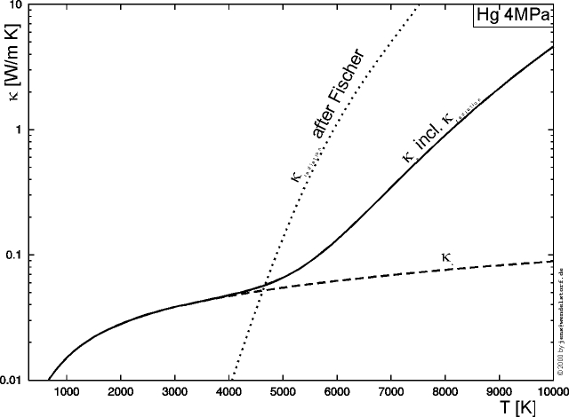 |
 |
 |
Another important application area of thermal plasma gas discharges are high pressure mercury discharge lamps. Currently, low power lamps at pressure levels around 4 MPa are introduced for car headlight systems and even ultra high pressure lamps (8-20 MPa) for data and video projection systems are under development or already available. The modelling of these lamps was reviewed by Dakin [36].
As shown in figure 5.44, the discharge is highly influenced by hydrodynamic phenomena. At atmospheric pressure, the flow field is dominiated by magnetic forces and at 80 atmospheres, the natural convection forces become of the same importance. Due to the higher radiative and conductive losses, the discharge also constricts at higher pressure levels.
One of the specifics of such arc discharges is the increasing role of
radiation transport phenomena with increasing pressure. Because detailed
radiation transport is not included into the model, such effects are
described by a radiative heat conductivity taking account of the optical
thick radiation emitted and reabsorbed within the discharge. Such a
radiative heat conductivity was computed
by Fischer [48] and was used by Giese [52]6:
| ||||||||||||||||
 |
For this work, the radiative heat conductivity was computed by Wilhelm [129], as shown in figure 5.43. The computed parameters for such a D1-lamp like discharge are provided in figure 5.45.
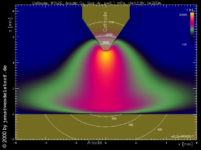 |
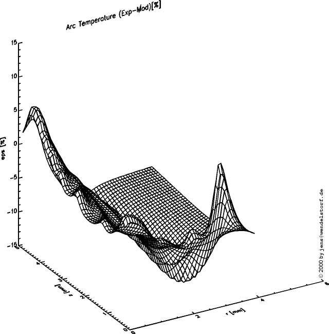 |
| Model/Exp | 100A | 200A |
| 100A | -6% | +5% |
| 200A | -18% | -7% |
The atmospheric pressure argon arc burning between a tungsten cathode and a flat anode is one of the arc configurations investigated in depth by experimental techniques like emission spectroscopy [22,54,57,65,118], Laser scattering [93] and Laser induced fluorescence [115]. Regarding the results of such spectroscopical arc temperature measurements, one has to take into account the small variation of arc temperature with arc current. In table 5.3, the mean deviation of measured and calculated arc temperature is provided for the LTE case. Comparing the computed 100A temperature map with the spectroscopical 200A temperature map gives a mean deviation still inside the experimental error bars.
Additionally, a number of independent groups have developed mathematical models for this so called standard welding arc [77]. A detailed review can be found in [127]. For this arc situtation, a number of arc electrode models was published [37,132,82]. Additionally, ambipolar diffusion and radiation transport was studied in depth [109,89]. Assuming LTE, the self consistent calculation of the arc electrode system is straightforward and the results agree with measured arc temperatures within the principal error.
While most experiments assume LTE for such a high current arc, there is strong evidence for non LTE effects near the electrodes [14], as well as in the arc column [58]. These calculations are in agreement with recent experiments [114,116]. Using the pLTE plasma electrode model in this work, one can investigate this problem in larger detail.
For the high pressure xenon model lamp (section 5.3.2), a comparison of this work (BS) with the results of a model developed by Wiesman [128] and Flesch [50] in the group of Prof. Neiger at Karlsruhe (LTI) is possible. The LTI model is based on a non-LTE electric conductivity equation, originally introduced by Fischer [48]. It solves the (LTE) heat conduction and current continuity equation on a very fine finite element grid.
| U[V] | UC[V] | E[V/m] | TC[K] | PC,¥ [W] | |
| BS | 19.4 | 9.9 | 622 | 3299 | 5.8 |
| LTI | 22.8 | 8.6 | 636 | 3474 | 6.0 |
As shown in table 5.4, the results are quite similar. Compared to the results presented in table 5.2, the BS-values were obtained including fluid flow and for rA = 0.3mm. The overall arc voltage may show better agreement with experiment for the LTI model, because of an underestimation of the anode fall by the model presented in this work. Because of the missing space charge layer model, the LTI values for the cathode tip temperatures may be found to be more inaccurate than the BS ones.
| U[V] | UC[V] | E[V/m] | TC[K] | PC,¥ [W] | |
| BS | 71.1 | 16.4 | 13400 | 3264 | 9.6 |
| LTI | 82.4 | 19.8 | 13900 | 3331 | 9.5 |
The same agreement is found by comparing the results obtained by the different models for a high pressure mercury short arc lamp (table 5.5). The differences in the arc voltage is a result of the different anode falls computed (0.9V for this model and 7.0V for the LTI one).
This comparison allows for a very important conclusion: The arc and electrode fall voltages mainly depend on the electrode work function and the temperature dependence of the electric conductivity. Including the most important effects governing the overall discharge self-consistently into the model, one will get similar results. These most important physical processes are:
While the model presented here (BS), was developed for maximum physical self consistency, even a model neglecting flow and sheath phenomena (LTI) may allow for a computation of the arc voltage current characteristics. This picture may change for the prediction of discharge parameters which are more sensitive to flow phenomena (see table 5.1).
The number of references describing a self-consistent arc modelling approach is limited to this work, the LTI approach and the work done at CSIRO in Australia (see e.g. [82]). For the model presented here, results in a pressure range of 0.1 to 8 MPa are available. The LTI model is restricted to pressures above 1 MPa, LTE discharges and neglects fluid flow phenomena. For the CSIRO model, only results for a high current atmospheric argon arc where published.
Taking into account modelling approaches with fit parameters (e.g. the peak current density at the cathode surface) or calculating only one specific region of the arc, there is a large amount of literature available. Most of these references deal with the TIG welding arc situation and are discussed in [127].
Some of the high pressure mercury lamp models presented in the literature provide results for a three dimensional flow situation [30,52]. Because of the missing cathode and anode layer model, the only measureable quantity provided is the arc temperature distribution. In [52], a reasonable number of different discharge situations was modeled. The results show the impact of natural convection, especially for the horizontal burning position and high pressure. Because the magnetic compression forces where neglected, the results are rather questionable both quantitatively and qualitatively, especially near the electrodes. No arc burning voltages were presented in [52].
This chapter has provided modelling results for a wide range of discharge parameters as well as a discussion of the influence of the individual physical effects on the overall discharge behaviour. It can be regarded as an in depth presentation of arc discharge properties based on ab initio mathematical modelling. Special emphasis was given to the impact of fluid flow and its specific driving forces.
Based on the results of a physical sensitivity analysis, an attempt was made to validate the model by comparision with experimental data. For discharges in LTE or near LTE, the available experimental data justifies the physical model.
A more detailed and accurate validation can be performed by enhancing the numerical calculation schemes to allow for the calculation of longer arcs and mode transitions using less computing time. The uncertainties of the electrode work function values and of the cross section and radiative data will require special strategies for an increase and test of the models accuracy.
|
In this chapter, the major achievements, especially in the realized modelling concept, are summarized, the application areas are sketched and finally some future developments are encouraged, followed by a final conclusion.
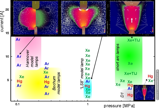 |
The modelling results were obtained by a large computer code (algorithmic complexity) using a large amount of computing time (logical depth). A comparison with the similar approaches cited above is restricted to the comparison of modelling results available for identical discharge configurations. It was performed for the model developed at the University of Karlsruhe (LTI,[50]).
The comparison of the results with available experimental data was provided for the quantitative measurement data sets available. The validation of the model was found to be limited by the required agreement of the computed and measured arc configuration, by the limited experimental accuracy and by the precision of the numerical solutions resulting from the numerical grid spacing and the inaccuracy of the input data, especially the cathode material work function.
As a conclusion, the LTE arc column and the cathode fall calculation was found to be as accurate as the experimental determination of cathode fall voltages and arc temperature distributions. The anode layer model may be regarded to provide a lower limit for the anode fall voltage and is the first self consistent one not neglecting space charge formation in front of the anode. A more detailed validation of the model will require a large number of accurate experiments obtained for discharges mainly in local thermodynamic equilibrium (LTE). This may also allow for a determination of parameters like the cathode work function by solving an inverse problem.
Within the limitations of the computing requirements and the experimental precision, the model was found to be suitable for a quantitative prediction of arc discharge data within a pressure range of 0.1 to 8 MPa and currents above 1 A.
The physical model has a large degree of self consistency by iteratively linking 2D plasma and 1D sheath models. Its success is based on the principle of applying different models to physically different regions, instead of trying to describe the overall discharge by a single set of equations. Compared to the LTI approach, the number of discretization points required is orders of magnitude smaller. The current implementation was optimized in terms of development time and thus wasting computing time by the missing solution adapted numerical mesh. This is not a disadvantage of the model itself. Additionally the transfer function approach for boundary layer modelling is very general and can the implemented into other existing computational fluid dynamics (CFD) or finite element (FEM) models.
The self consistent locally defined space charge layer model may be regarded as the most important part of the approach, but the overall realization of the scheme was clearly the most complex part of this work.
The range of possible applications of such an ab initio predictive modelling approach is as wide as the application area of arc discharges itself. While the actual model is (numerically) restricted to stationary direct current (DC) discharges with cylindrical symmetry, the first applications will lie in the field of high intensity discharge (HID) lamps. One of the direct application areas are high pressure short arc lamps used for projection devices, searchlights, laser pumping and other areas where large light intensities are required. Such products may be improved by modelling and/or model enhanced experimental optimization. Especially for high pressure mercury discharges, additional radiation transport modelling will be required. As a conclusion, the model may change the way of light source development from trial and error to computational prediction and optimization.
Electric arc discharges are also applied as energy sources for high temperature material processing. New cutting, welding and spraying torches, as well as other new arc applications may be developed on the basis of the model. Currently, the optimization of DC tungsten inert gas welding processes (TIG/GTAW), as well as plasma arc welding (PAW) is in reach of the model. A few enhancements of the numerical procedures will also allow for an optimization of arc furnaces for metal and mineral processing and waste destruction. More sophisticated enhancements of the numerics are required for modelling transient arc discharges, which can be found in circuit breakers and switches.
The possible enhancements of the model can be divided into three different fields. First, the physical model can be optimized by implementing the generalized Ohms law, ambipolar diffusion within the arc core, other diffusion and demixing processes and a more detailed radiation transport model. Second, the numerical solution has to be optimized by transferring the approach to a commercial CFD software package. Finally, the problem of bifurcations (mode transitions), multiple solution hysteresis and all other aspects of discharge complexity can be addressed by further fundamental research. All these enhancements strongly interact with each other and have to be carefully planned and weighted against the available development resources.
Parallel to the model enhancement, validation experiments have to be performed. It is proposed to optimize the input parameters (cathode work function, cross section and radiative data) for a best fit to one set of experimental data and to test the extrapolation capability of the model by comparison with a second set of experimental data.
Thermal plasma gas discharges (electric arcs) are complex self organizing dissipative physical systems. For specific parameter sets representing an increasing survival pressure, the discharge reorganizes itself to a more sophisticated spatial structure (symmetry breaking) or self organized criticality (constricted electrode attachment).
While such complex natural phenomena are actually mostly unpredictable, this work has shown the possibility of quantitative and ab initio computation of complete and really existing discharge configurations. The physical desription was found to be more general than the actual numerical implementation, which is limited to the stationary radial symmetric case.
The final conclusion is the practical predictability of this type of gas discharges by mathematical modelling. It was achieved by a proper balance of physical understanding and application oriented numerical software development. The computational effort was 1011¼12 floating point operations per discharge configuration.
| Danksagung |
Mein besonderer Dank gilt meinem Doktorvater, Herrn Prof. Dr. G. Simon für die Möglichkeit der Anfertigung dieser Arbeit, die angenehme Betreuung und die zahlreichen Anregungen. Seinem Andenken als Wissenschaftler und herausragende Persönlichkeit ist diese Dissertation gewidmet.
Herrn Prof. Dr. U. Motschmann danke ich für die durch den Tod von Prof. Simon veranlaßte Übernahme der Mentorenschaft dieser Arbeit. Seine Verbesserungsvorschläge und sein Engagement haben wesentlich zur Qualität der Darstellung beigetragen und mir die Fertigstellung unter schwierigen Umständen ermöglicht.
Herrn Prof. Dr. M. Kock und Herrn Prof. Dr. J. Mentel danke ich für die Bereitschaft zur Übernahme der Koreferate. Ihnen und den anderen Mitgliedern der von Herrn Prof. Dr. W. Bötticher und Herrn Prof. Dr. K. Günther koordinierten Forscherverbünde zum Thema Lampenkatoden sei an dieser Stelle für die Möglichkeit der Mitwirkung an diesem äußerst fruchtbaren Projekt und die zahlreichen Diskussionen gedankt.
Herzlich danken möchte ich mich auch den Kollegen in Europa, USA und Australien für die vielen konstruktiven wissenschaftlichen Diskussionen. Diese Arbeit ist erst durch die freie Kommunikation mit den anderen auf diesem Gebiet tätigen Forschern möglich geworden.
Meine Dankbarkeit gilt besonders meiner Freundin Doris und meinen Eltern für ihre Geduld und Unterstützung.
Die Ergebnisse dieser Arbeit wurden im Rahmen des vom BMBF geförderten Forscherverbundes "Lampenkatoden" (13N7105/9) berechnet. Die notwendigen Erfahrungen und Berechnungsverfahren entstanden in den Jahren 1994 bis 1999 während meiner Tätigkeit am Institut für Schweißtechnik der TU-Braunschweig unter der Leitung von Herrn Prof. Dr. H. Wohlfahrt. Er und seine Mitarbeiter und Mitarbeiterinnen haben die Durchführung dieser Arbeit erst möglich gemacht. Alle hier nicht namentlich genannten Freunde und Kollegen mögen mir verzeihen, daß ich an dieser Stelle nur noch Frau Dr. B. Rethfeld und Herrn R. Montero erwähne, die im Rahmen ihrer Diplomarbeit einen Beitrag zum Gelingen dieser Arbeit geleistet haben.
Wissenschaftliche Veröffentlichungen und Tagungsbeiträge
allgemeiner Art:
von Aluminiumlegierungen.
DVS-Berichte, Bd.170 (1995), S.96-99
4tes ifs-Kolloqium, IHK Braunschweig, 5.7.97.
3tes ifs-Kolloqium, Braunschweig, 28-29.6.96.
Stabilisierung des Schweißlichtbogens,
Verhandl. DPG (VI), Bd.27 (1992), S.1273
Verhandl. DPG (VI), Bd.26 (1991), S.305
auftretenden Raumladungsschicht.
Verhandl. DPG (VI), Bd.25 (1990), S.343
1 [(D)/(Dt)](¼) = [(¶)/(¶t)](¼) + [(v)\vec] ·[(Ñ)\vec] (¼)
2describing the relation of momentum diffusity to thermal diffusity [4].
3With decreasing size of the layer, there are circumstances where the temperature split can be modeled by the cathode layer model only.
4With decreasing total current the discharge can become dominated by the requirement to heat the cathode to thermionic emission temperatures - the cathode attachment thus can be calculated by a sheath-cathode model [27].
5The work function of pure tungsten is estimated to be 4.35¼4.65 eV.
6like all quantities in this work, given in SI Units.